Decision Tree: Classification methods
Introduction
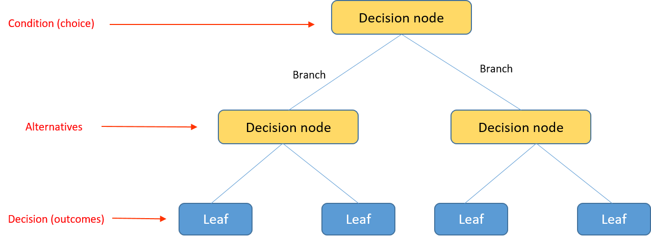
Decision Tree is a Supervised learning technique that can be used for both classification and Regression problems, but mostly it is preferred for solving Classification problems. It is a tree-structured classifier consisting of a root node, branches, internal nodes, and leaf nodes, where internal nodes represent the features of a dataset, branches represent the decision rules and each leaf node represents the outcome.
The decision rules are generally in form of if-then-else statements. The deeper the tree, the more complex the rules and fitter the model.
- Root Node: This is the starting point of the tree. It represents the entire dataset and is where the first decision is made. The root node corresponds to the feature that best splits the data into distinct groups, maximizing the homogeneity of the target variable within each group.
- Internal Nodes/Decision Nodes: These nodes represent features or attributes that are used to partition the data further. Each internal node corresponds to a decision based on a specific feature, leading to one or more branches.
- Branches: Branches emanate from internal nodes and represent the possible outcomes of the decision based on the feature at that node. Each branch corresponds to a specific value or range of values of the feature being evaluated.
- Leaf Nodes: These are the terminal nodes of the tree, where no further splitting occurs. Each leaf node represents a class label (in classification) or a predicted value (in regression). The decision tree algorithm aims to make the predictions at the leaf nodes as accurate as possible based on the features and their values.
Example-1
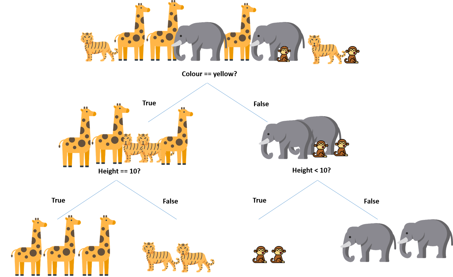
Suppose there are different animals, and you want to identify each animal and classify them based on their features. We can easily accomplish this by using a decision tree.

The following is a cluttered sample data set with high entropy:
| Color | Height | Label |
|---|---|---|
| Grey | 10 | Elephant |
| Yellow | 10 | Giraffe |
| Brown | 3 | Monkey |
| Grey | 10 | Elephant |
| Yellow | 4 | Tiger |
We have to determine which features split the data so that the information gain is the highest. We can do that by splitting the data using each feature and checking the information gain that we obtain from them. The feature that returns the highest gain will be used for the first split. Let's consider following features into consideration:
| Condition |
|---|
| Color == Yellow |
| Height >= 10 |
| Color == Brown |
| Color == Grey |
| Diameter <10 |
We’ll use the information gain method to determine which variable yields the maximum gain, which can also be used as the root node.
- Suppose
Color == Yellowresults in the maximum information gain, so that is what we will use for our first split at the root node - The entropy after splitting should decrease considerably. However, we still need to split the child nodes at both the branches to attain an entropy value equal to zero.
- We will split both the nodes using
heightvariable andheight > 10andheight < 10as our conditions. - The decision tree below can now predict all the classes of animals present in the data set
Working Principle
In a decision tree, for predicting the class of the given dataset, the algorithm starts from the root node of the tree. This algorithm compares the values of root attribute with the record (real dataset) attribute and, based on the comparison, follows the branch and jumps to the next node. For the next node, the algorithm again compares the attribute value with the other sub-nodes and move further. It continues the process until it reaches the leaf node of the tree.
The algorithm works by recursively partitioning the data into subsets based on the most significant attribute at each node using the Attribute Selection Measure (ASM). This process continues until the subsets at a node have the same target variable or reach a specified maximum depth.
The working principle of a decision tree involves the following steps:
- Feature Selection: The algorithm evaluates different features in the dataset to determine the best feature that splits the data into distinct groups. It selects the feature that maximizes the homogeneity (or purity) of the target variable within each group.
- Splitting: After selecting the best feature, the algorithm splits the dataset into subsets based on the values of that feature. Each subset corresponds to a different branch of the tree.
- Recursive Partitioning: This process of feature selection and splitting continues recursively for each subset until a stopping criterion is met. Common stopping criteria include reaching a maximum tree depth, having a minimum number of samples in a node, or no further improvement in purity.
- Leaf Node Assignment: Once the recursive partitioning process reaches a stopping point, the algorithm assigns a class label (in classification) or a predicted value (in regression) to each leaf node based on the majority class or average target variable value of the samples in that node.
- Prediction: To make predictions for new data points, the algorithm traverses the decision tree from the root node down to a leaf node, following the decision rules at each internal node based on the features of the data point. The prediction at the leaf node reached by the traversal is then assigned to the data point.
Splitting criteria in Decision trees: Attribute Selection Measure (ASM)
The splitting criteria in decision trees are used to determine how the data should be partitioned at each node of the tree. Attribute Selection Measure (ASM) is a term often used in the context of decision trees, specifically regarding the selection of the best attribute to split the data at each node. ASM refers to the criterion or metric used to evaluate and rank the attributes based on their effectiveness in partitioning the data and improving the homogeneity of the resulting subsets.
What is Attribute Selection Measure (ASM)?
ASM is a criterion or metric used in decision tree algorithms to assess the importance of different attributes in making splitting decisions. It helps determine which attribute should be chosen as the splitting criterion at each node of the decision tree. The attribute with the highest ASM score is typically selected for splitting, as it leads to more informative and discriminative splits.
Why is ASM important?
ASM plays a crucial role in the construction of decision trees by guiding the algorithm in selecting the most relevant attributes for partitioning the data. By choosing attributes with high ASM scores, decision trees can effectively divide the dataset into subsets that are more homogeneous with respect to the target variable. This, in turn, leads to the creation of accurate and interpretable decision tree models.
Common ASM Methods:
Several methods exist for calculating ASM, each with its own strengths and considerations. Some common ASM methods include:
- Information Gain (Entropy): Information gain measures the reduction in entropy (or uncertainty) achieved by splitting the data based on a particular feature. The goal is to select the feature that maximizes information gain, thereby improving the purity of the resulting subsets. Higher information gain implies better separation of classes or reduced randomness in the subsets.
Working principle:The decision tree algorithm evaluates each feature and calculates the entropy of the dataset before and after splitting based on that feature. Information gain is then computed as the difference between the initial entropy and the weighted sum of entropies of the resulting subsets.
Formulation:Entropy is a measure of randomness or uncertainty in a dataset. Mathematically, it is defined as:
$$H(X) = - \sum_{i=1}^n p_i \log_2(p_i)$$ where:- \(H(X)\) is the entropy of the dataset \(X\).
- \(p_i\) is the probability of class \(i\) in the dataset.
- \(n\) is the total number of classes.
Information gain is used to select the best feature for splitting the data in decision trees. It measures the reduction in entropy (or increase in purity) achieved by splitting the data based on a particular feature. Mathematically, information gain is calculated as:
$$\text{Information Gain} = H(X) - \sum_{j=1}^m \frac{N_j}{N} H(X_j).$$which can also be written as: Information Gain= Entropy(S)- [(Weighted Avg) \(\times\) Entropy(each feature)]
where:- \(H(X)\) is the entropy of the original ataset \(X\).
- \(m\) is the number of subsets after splitting based on the feature.
- \(N_j\) is the number of samples in subset \(i\).
- \(N\) is the total number of samples in the original dataset.
- \(H(X_j)\) is the entropy of subset \(j\).
Interpreation:Higher information gain indicates that splitting based on a certain feature leads to more homogeneous subsets with respect to the target variable. In other words, it signifies that the feature provides more discriminatory power for classification.
Application: Information gain is commonly used in decision tree algorithms such as ID3 (Iterative Dichotomiser 3) and C4.5 (successor to ID3) for building classification trees.
Example
Let’s understand decision trees with the help of an dataset of last 10 days:
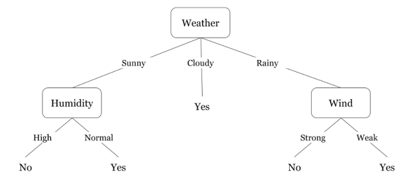
Day Weather Teperature Humidity Wind Play? 1 Sunny Hot High Weak No 2 Cloudy Hot High Weak Yes 3 Sunny Mild Normal Strong Yes 4 Cloudy Mild High Strong Yes 5 Rainy Mild High Strong No 6 Rainy Cool Normal Strong No 7 Rainy Mild High Weak Yes 8 Sunny Hot High Strong No 9 Cloudy Hot Normal Weak Yes 10 Rainy Mild High Strong No Decision trees are nothing but a bunch of if-else statements in layman terms. It checks if the condition is true and if it is then it goes to the next node attached to that decision.
In the diagram below, the tree will first ask what is the weather? Is it sunny, cloudy, or rainy? If yes then it will go to the next feature which is humidity and wind. It will again check if there is a strong wind or weak, if it’s a weak wind and it’s rainy then the person may go and play.
Suppose we have a dataset with the following target variable (class labels) and one attribute:
Day Attribute (feature) Play? 1 Sunny No 2 Cloudy Yes 3 Sunny Yes 4 Cloudy Yes 5 Rainy No 6 Rainy No 7 Rainy Yes 8 Sunny No 9 Cloudy Yes 10 Rainy =No We can cluttered the dataset as follows:
Counts(Yes) Counts(No) Sunny 1 2 Cloudy 3 0 Rainy 1 3 Similalry we can create a table for the Temperature, Humidity, and Wind,features.
Now, let's calculate the entropy of the target variable "Play?" and then compute the Information Gain for each attribute (feature).
- Step-1: Calculate the entropy of the target variable "Play?":
Total instances (sample): \(n =10\)
Number of "Yes" instances (positive): \(p_{\text{Yes}} = 5\)
Number of "No" instances (negative): \(p_{\text{No}} = 5\)
Entropy (H(play?)):
$$H(Play?) = - \left(\frac{5}{10} \log_2\frac{5}{10}+\frac{5}{10} \log_2\frac{5}{10}\right) = -(-0.5 -0.5) =1$$ - Step 2: Calculate Information Gain for each feature:
Sunny:
- Total instances with "Cloudy": \(n =3\)
- Number of "Yes" instances (positive) with "Sunny": \(p_{\text{Yes,Sunny}}=1\)
- Number of "No" instances (negative) with "Sunny": \(p_{\text{No,SUnny}}=2\)
- Entropy for "Sunny" i.e. \(H(Sunny) = -\left(\frac{1}{3} \log_2\frac{1}{3}+\frac{2}{3} \log_2\frac{2}{3}\right) =0.918\)
- Information Gain i.e. \(IG(\text{Play?, Sunny}) = 1-\frac{3}{10}\times 0.918 =0.7246\). Similalry, we can calculate entropy and information Gain for "Cloudy" and "Rainy".
Cloudy:
- Total instances with "Cloudy": \(n =3\)
- Number of "Yes" instances (positive) with "Cloudy": \(p_{\text{Yes,Cloudy}}=3\)
- Number of "No" instances (negative) with "Cloudy": \(p_{\text{No,Cloudy}}=0\)
- Entropy for "Cloudy" i.e. \(H(Cloudy) = -\left(\frac{3}{3} \log_2\frac{3}{3}+\frac{0}{3} \log_2\frac{0}{3}\right) =0\)
- Information Gain i.e. \(IG(\text{Play?, Cloudy}) = 1-\frac{3}{10}\times 0 =1\).
Rainy:
- Total instances with "Rainy": \(n =4\)
- Number of "Yes" instances (positive) with "Rainy": \(p_{\text{Yes,Rainy}}=1\)
- Number of "No" instances (negative) with "Rainy": \(p_{\text{No,Rainy}}=3\)
- Entropy for "Rainy" i.e. \(H(Rainy) = -\left(\frac{1}{4} \log_2\frac{1}{4}+\frac{3}{4} \log_2\frac{3}{4}\right) =0.8113\)
- Information Gain i.e. \(IG(\text{Play?, Rainy}) = 1-\frac{4}{10}\times 0.8113 =0.6755\).
Now we can calculate the weighted entropy for weather feature:
$$H_{\text{Weather}} = \frac{3}{10} \times H_{\text{Sunny}} + \frac{3}{10} \times H_{\text{Cloudy}} + \frac{4}{10} \times H_{\text{Rainy}} = \frac{3}{10} \times 0.918 + \frac{3}{10} \times 0 + \frac{4}{10} \times 0.8113 =0.5999$$Similalry, Information gain:
$$IG_{\text{Weather}} = H- H_{\text{Weather}} = 1-0.5999=0.4001$$
Similarly, calculate information gain for other features: Temperature, Humidity, Wind. This process will help us determine which feature provides the most Information Gain, indicating its importance for splitting the dataset in the decision tree.
- Gini Index (Impurity): Gini impurity measures the probability of misclassifying a randomly chosen sample if it were labeled according to the class distribution in the dataset. The goal is to select the feature that minimizes Gini impurity, thereby improving the homogeneity of the resulting subsets. Lower Gini impurity implies purer subsets with fewer mixed-class samples.
Working Principle: Similar to information gain, the decision tree algorithm evaluates each feature and calculates the Gini impurity of the dataset before and after splitting based on that feature. The feature with the lowest Gini impurity (or highest purity) is selected for splitting. Mathematically, Gini impurity is calculated as:
$$G(X) = 1- \sum_{i=1}^n p_i^2$$ where:- \(G(X)\) is the Gini impurity of the dataset \(X\).
- \(p_i\) is the probability of class \(i\) in the dataset.
- \(n\) is the total number of classes.
Interpretation:Lower Gini impurity indicates that splitting based on a certain feature leads to more homogeneous subsets with respect to the target variable. It signifies that the feature effectively separates the classes in the dataset.
Application:Gini impurity is commonly used in decision tree algorithms such as CART (Classification and Regression Trees) for building both classification and regression trees.
- Gain Ratio: Gain Ratio is a modification of Information Gain that aims to overcome its bias towards attributes with a large number of distinct values. It penalizes attributes with many distinct values, thereby helping to prevent overfitting.
Formula:
$$\text{Gain Ratio} = \frac{\text{Information Gain}}{\text{Split Information}}$$Explanation:Gain Ratio adjusts Information Gain by considering the intrinsic information of each attribute. It divides the Information Gain by the Split Information to normalize the gain by the attribute's intrinsic information. This normalization helps in avoiding the bias towards attributes with many distinct values.
- Chi-Square Test:Chi-Square Test evaluates the independence between attributes and the target variable by comparing the observed distribution of class labels in each subset to the expected distribution. It helps determine whether the splits based on a particular attribute are statistically significant.
Formula:The Chi-Square Test statistic is calculated as follows:
$$\chi^2 = \sum_{i=1}^k \frac{(O_i - E_i)^2}{E_i}$$ where:- \(\chi^2\) is the Chi-Square test statistic.
- \(O_i\) is the observed frequency of class \(i\) in the subset.
- \(E_i\) is the expected frequency of class \(i\) based on the overall distribution.
Explanation: Chi-Square Test compares the observed frequencies of class labels in each subset to the expected frequencies based on the overall distribution. A higher Chi-Square Test statistic indicates a greater difference between the observed and expected frequencies, suggesting that the splits based on the attribute are more informative and significant.
Each of these methods evaluates attributes based on different criteria, such as the reduction in entropy, impurity, or independence between attributes and the target variable. The choice of ASM method depends on the specific characteristics of the dataset and the problem being addressed.
Application of ASM
ASM is widely used in decision tree algorithms such as ID3, C4.5, and CART for attribute selection. These algorithms leverage ASM to determine the optimal splitting criteria at each node, leading to the creation of decision trees that effectively capture the underlying patterns and relationships in the data.
In conclusion, Attribute Selection Measure (ASM) is a fundamental concept in decision tree algorithms, guiding the selection of attributes for splitting the data at each node. By evaluating and ranking attributes based on their effectiveness in partitioning the data, ASM helps construct decision trees that are accurate, interpretable, and well-suited for a variety of machine learning tasks.
Example-1: User dataset
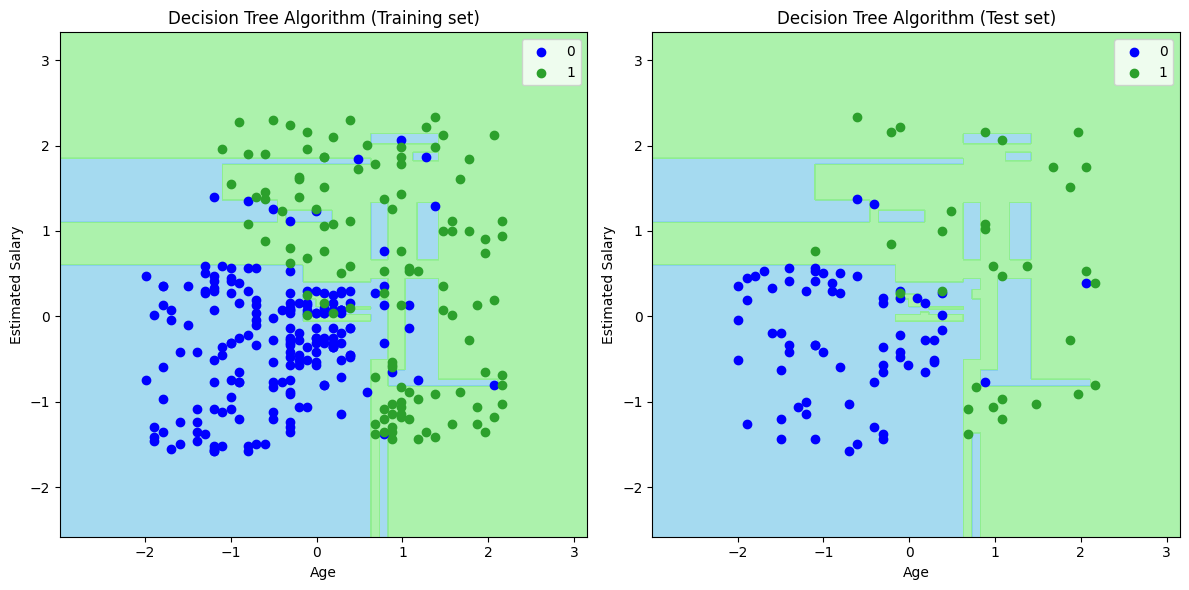
In this example, we again consider the user dataset similar to what we used in the case of Navive-Bayes and the KNN-algorithm. We first use the feature and target, then use the train_test_split to create the train and test datasets. In the final step, we instantiate the classifer using ecisionTreeClassifier and build our model using the train datset. In the end, we visualize how our model performs on the train and test datsets. The detailed notebook is available at my Github repo and the code is available in the Jupyter notebook at my repo.
                    import pandas as pd
                    import numpy as np
                    import matplotlib.pyplot as plt

                    df_user =  pd.read_csv('User_Data.csv')


                    # Importing the dataset
                    X = df_user.iloc[:, [2, 3]].values
                    y = df_user.iloc[:, 4].values

                    # Splitting the dataset into the Training set and Test set
                    from sklearn.model_selection import train_test_split
                    X_train, X_test, y_train, y_test = train_test_split(X, y, test_size = 0.25, random_state = 0)

                    # Feature Scaling
                    from sklearn.preprocessing import StandardScaler
                    sc = StandardScaler()
                    X_train = sc.fit_transform(X_train)
                    X_test = sc.transform(X_test)

                    #Fitting Decision Tree classifier to the training set

                    from sklearn.tree import DecisionTreeClassifier
                    classifier = DecisionTreeClassifier(criterion='entropy', random_state=0)
                    classifier.fit(X_train, y_train)

                    # Importing libraries
                    import matplotlib.pyplot as plt
                    from matplotlib.colors import ListedColormap

                    # Set up the figure with two subplots in one row and two columns
                    fig, axes = plt.subplots(1, 2, figsize=(12, 6))

                    # Visulaizing the training set result
                    x_set, y_set = X_train, y_train
                    X1, X2 = np.meshgrid(np.arange(start=x_set[:, 0].min() - 1, stop=x_set[:, 0].max() + 1, step=0.01),
                                        np.arange(start=x_set[:, 1].min() - 1, stop=x_set[:, 1].max() + 1, step=0.01))
                    axes[0].contourf(X1, X2, classifier.predict(np.array([X1.ravel(), X2.ravel()]).T).reshape(X1.shape),
                                    alpha=0.75, cmap=ListedColormap(['#87CEEB', '#90EE90']))
                    axes[0].set_xlim(X1.min(), X1.max())
                    axes[0].set_ylim(X2.min(), X2.max())

                    for i, j in enumerate(np.unique(y_set)):
                        axes[0].scatter(x_set[y_set == j, 0], x_set[y_set == j, 1],
                                        c=ListedColormap(['#0000FF', '#2ca02c'])(i), label=j)

                    axes[0].set_title('K-NN Algorithm (Training set)')
                    axes[0].set_xlabel('Age')
                    axes[0].set_ylabel('Estimated Salary')
                    axes[0].legend()

                    # Visulaizing the test set result
                    x_set, y_set = X_test, y_test
                    X1, X2 = np.meshgrid(np.arange(start=x_set[:, 0].min() - 1, stop=x_set[:, 0].max() + 1, step=0.01),
                                        np.arange(start=x_set[:, 1].min() - 1, stop=x_set[:, 1].max() + 1, step=0.01))
                    axes[1].contourf(X1, X2, classifier.predict(np.array([X1.ravel(), X2.ravel()]).T).reshape(X1.shape),
                                    alpha=0.75, cmap=ListedColormap(['#87CEEB', '#90EE90']))
                    axes[1].set_xlim(X1.min(), X1.max())
                    axes[1].set_ylim(X2.min(), X2.max())

                    for i, j in enumerate(np.unique(y_set)):
                        axes[1].scatter(x_set[y_set == j, 0], x_set[y_set == j, 1],
                                        c=ListedColormap(['#0000FF', '#2ca02c'])(i), label=j)

                    axes[1].set_title('K-NN Algorithm (Test set)')
                    axes[1].set_xlabel('Age')
                    axes[1].set_ylabel('Estimated Salary')
                    axes[1].legend()

                    plt.tight_layout()
                    plt.show()
Example-2: Titanic dataset
In this example, we will use Titanic dataset. This dataset is available at Kaggle. Lets do this example step by step:
- Step-1: Load the dataset and selecting the feature and taget vairable:
Since Column 'Sex' contains either 'Male' or 'Female', we are going to change them to numerical values. Similary droping the not needed columns in our analysis and ignorning the NaN values:import pandas as pd import matplotlib.pyplot as plt %matplotlib inline df = pd.read_csv('titanic.csv') -
In the next step, we need to create the dummy columns for our target variable. The dummy/indicator variables are used for converting the categoriecal variables. For this prupose, we use# checnging the categorical values for Sex to 0 or 1. df['Sex'] = df['Sex'].map({'male': 0, 'female': 1}) # we dont need the Cabin column in our case df.drop(['Cabin', 'Name', 'Ticket'], axis=1, inplace=True) # droping the NaN values df.dropna(inplace=True)get_dummiesclass, which creates new columns for each unique value in the categorical column, with binary values indicating the presence or absence of each value in the original column.
Now the X and y variables can be found as:df = pd.get_dummies(df, columns=['Embarked'])X = df.drop('Survived', axis=1) y = df['Survived'] - Train-test and model building
Again us instantiate our classifierfrom sklearn.model_selection import train_test_split X_train, X_test, y_train, y_test = train_test_split(X, y, test_size=0.25, random_state=42)DecisionCLassifierfrom the sub-modulesklearn.tree. Here we choose the depth of the tree.
The socre from the train and test datasets can be found byfrom sklearn.tree import DecisionTreeClassifier model = DecisionTreeClassifier(max_depth = 3, random_state=42) model.fit(X_train, y_train)model.score(X_train, y_train)andmodel.score(X_test, y_test)which gives the socre for the two datsets 0.8370786516853933 and 0.7528089887640449. The analysis of the score on the training set and on the test set allows to identify the overfitting. Indeed, the score on the training test is higher than the test score. To overcome this problem we will add another parameter:min_samples_leaf. This parameter indicates the minimum number of samples required for a node separation. So, if there are not enough samples, the node will be a leaf (a final node). The parametersmax_depthandmin_samples_leafare two essential parameters to avoid overfitting.from sklearn.tree import DecisionTreeClassifier model_min_samples = DecisionTreeClassifier(max_depth = 3, min_samples_leaf = 25, random_state=42) model_min_samples.fit(X_train, y_train)Now in this case, we found that accuracies for the train and test datsets are reduced and are
0.8258426966292135and0.7471910112359551respectively.Although the score on the training set has slightly decreased, we notice that the gap between the score on the training set and the score on the test set is reduced. We therefore decide to continue with this model which generalizes better on the data it does not know.
- The interpretation of the model:
One of the strong points of decision trees is the simplicity of interpreting how they work. In the same way that we analyzed our regression tree, we can analyze our classification tree. With this study, we want to know which variables are the most important for the model and which thresholds it uses to make its predictions.
                            from sklearn.tree import plot_tree

                            fig, ax = plt.subplots(figsize=(40, 20))

                            plot_tree(model_min_samples,
                                    feature_names=[
                                        'Pclass', 'Sex', 'Age', 'SibSp', 'Parch', 'Fare', 'Embarked_C',
                                        'Embarked_Q', 'Embarked_S'
                                    ],
                                    class_names=['Died', 'Survived'],
                                    filled=True,
                                    rounded=True)

                            plt.show()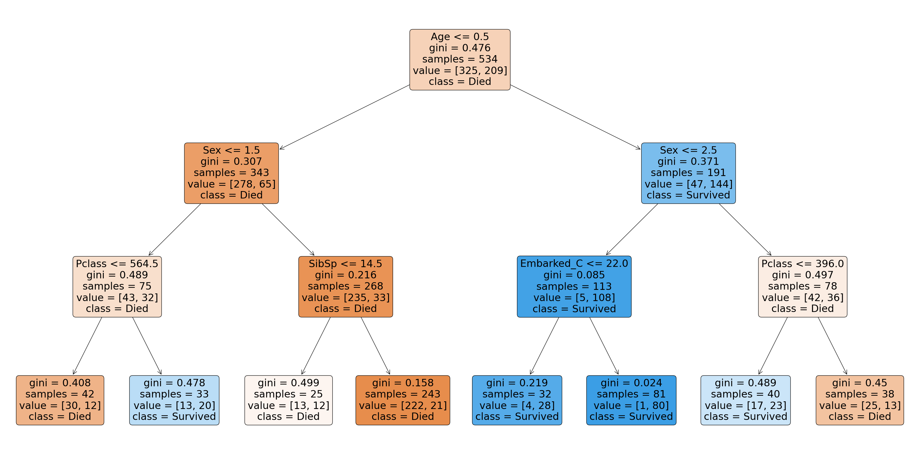
- The root node, the node at the top of the tree, contains all the samples of the training set, there are 534 samples: samples=534.
The first test that will be performed corresponds to Sex < = 0.5. As a reminder, Sex is a binary variable, it is equal to 0 when the individual is a man, 1 when it is a woman. We then look at the value for each sample. All the samples for which the variable Sex is 0, go in the left child node, if not in the right child node. More simply, all men go in the left child node, all women in the right child node.
The parameter value indicates the distribution of classes in y_train before any separation. We have initially 325 individuals who are dead and 209 who are alive. The class parameter indicates which is the majority class. Here it is the class 0 "Died": class = Died.
Finally, for a classification problem, the error is calculated using the Gini criterion. This criterion is between 0 and 0.5. The higher this criterion is, the more heterogeneous the node is and the lower the criterion is, the more homogeneous it is. A node is homogeneous when it contains only samples of one class, the Gini criterion is equal in this case to 0.
The objective of our model is to separate our classes as well as possible, so we want to end up with nodes as homogeneous as possible. Finally, the more homogeneous a leaf will be, with a low Gini criterion, the better the model will perform.
- We remind that the child nodes are the intermediate nodes of the tree. In the first left child node, we retrieve all the male individuals. There are 343 males in the training set (samples=343). The application of the condition described in the root node, allows us to reduce the Gini score by almost 0.169, we go from 0.476 to 0.307. The application of this condition has increased the homogeneity of the node. In this child node, there are more people who died than survived (278 > 65). The majority class is Died.
- The separations follow until the leaves, the terminal nodes, are obtained. The predicted class for the samples belonging to the leaf is the majority class. The color code is as follows: Orange when the majority class is class 0, Blue when it is class 1. The intensity of the color depends on the value of the Gini criterion, the lower it is the more intense the colors are. For the leftmost leaf, we have a Gini criterion equal to 0.5. There are 50 samples and the distribution is 25 samples belonging to class 0 and 25 samples to class 1. The node is therefore perfectly heterogeneous. This means that the model is wrong for 25 individuals, i.e. 50% of the samples of this sheet.
- The root node, the node at the top of the tree, contains all the samples of the training set, there are 534 samples: samples=534.
Finally, the variables that enabled the classification of the samples, ranked in order, are "Sex", "Pclass", "Age" and "Fare". The higher a variable is placed in the tree, the more important it played a role in the classification.
But how to quantify the role of each variable?
Instead of displaying the tree, or in addition to this analysis, it is possible to study the "feature importances" of the model. This attribute of the model class, called feature_importances_, allows to classify the variables according to the role they played in the prediction choices of the model. The sum of these values is 1.
The importance of a variable is calculated from the decrease in node impurity weighted by the probability of reaching the node. And the probability of reaching the node is obtained by dividing the number of samples reaching the node by the total number of samples.
Finally, the higher the importance value, the more important the variable.
                    X_importances = pd.DataFrame({
                        "Variables": X.columns,
                        "Importance": model_min_samples.feature_importances_
                        }).sort_values(by='Importance', ascending=False)


                    X_importances.nlargest(4, "Importance").plot.bar(x="Variables",
                        y="Importance",
                        figsize=(15, 5),
                        color="#4529de");
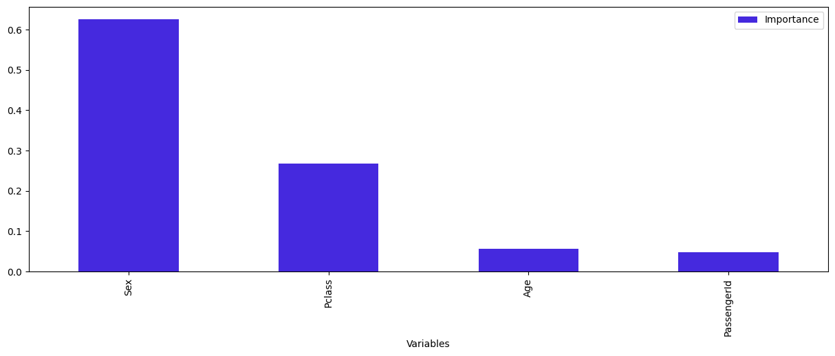
From these elements, we are able to decide on the accuracy of the expression "women and children first" (within the context of the data we have at our disposal). The women are indeed among the people who survived most after the disaster. The Sex variable is the most important one in the model. Nevertheless, even if age is among the three most important variables in the tree, a more precise analysis of the tree does not allow us to validate this assertion.
References
- Github repo with codes.
- Confusion matrix details.
- My github Repositories on Remote sensing Machine learning
- A Visual Introduction To Linear regression (Best reference for theory and visualization).
- Book on Regression model: Regression and Other Stories
- Book on Statistics: The Elements of Statistical Learning
- Naïve Bayes Classifier Algorithm, JAVAPoint.com
- https://www.colorado.edu/amath/sites/default/files/attached-files/ch12_0.pdf
- One of the best description on Linear regression.
Some other interesting things to know:
- Visit my website on For Data, Big Data, Data-modeling, Datawarehouse, SQL, cloud-compute.
- Visit my website on Data engineering

