In the realm of machine learning, classification problems involve the task of categorizing input data into distinct classes or categories based on certain features or attributes. This fundamental problem finds widespread
applications across various domains, ranging from medical diagnosis and sentiment analysis to image recognition and spam detection.
Among the plethora of algorithms available for classification tasks, logistic regression stands out as a versatile and widely-used method. Despite its name, logistic regression is not used for regression problems but
rather for binary classification, where the goal is to predict the probability of an observation belonging to a particular class.
Importance of Logistic Regression
Logistic regression holds significant importance in the field of machine learning for several reasons. Firstly, it provides a simple yet powerful framework for modeling the relationship between input features and the
likelihood of belonging to a particular class. This makes it particularly suitable for scenarios where interpretability and explanatory power are crucial.
Secondly, logistic regression offers robustness and efficiency, making it well-suited for both small and large-scale classification tasks. Its computational simplicity and ability to handle high-dimensional data make
it a popular choice for real-world applications.
Need of Logistic Regression
Linear regression and logistic regression are both widely used techniques in machine learning, but they serve different purposes and are suited for different types of problems.
Linear Regression: Linear regression is used for predicting continuous outcomes. It models the relationship between a dependent variable and one or more independent variables by fitting a
linear equation to the observed data points. The output of linear regression is a continuous value, making it suitable for regression tasks where the target variable is numeric.
Logistic Regression: Logistic regression, on the other hand, is specifically designed for binary classification tasks, where the outcome variable is categorical and has two possible
classes (e.g., yes/no, spam/not spam). Unlike linear regression, logistic regression models the probability that a given input belongs to a particular class. It uses the logistic function (also known as the
sigmoid function) to map input features to a probability value between 0 and 1, making it suitable for classification problems.
Advantages of Logistic Regression
Logistic regression offers several advantages that make it a popular choice for binary classification tasks:
Simple and Interpretable: Logistic regression models are relatively simple and easy to interpret compared to more complex algorithms like neural networks. The coefficients of logistic regression can
be directly interpreted in terms of the impact of each feature on the predicted probability of the target class.
Efficient Training and Inference: Logistic regression models are computationally efficient to train and make predictions with, especially for large datasets. They require less computational resources
compared to more complex models, making them suitable for real-time applications.
Probabilistic Interpretation: Logistic regression provides probabilistic outputs, allowing users to understand the uncertainty associated with each prediction. This probabilistic interpretation is useful
for decision-making and risk assessment in various domains.
Scope of Applications
Logistic regression finds applications across various fields due to its simplicity, interpretability, and effectiveness in binary classification tasks. Some common applications include:
Medical Diagnosis: Predicting the likelihood of disease occurrence based on patient symptoms and medical history.
Credit Risk Assessment: Assessing the risk of default for loan applicants based on financial and demographic factors.
Marketing Analytics: Predicting customer churn or likelihood of response to marketing campaigns based on customer behavior and demographic information.
Fraud Detection: Identifying fraudulent transactions based on patterns and anomalies in financial data.
Sentiment Analysis: Classifying text data (e.g., customer reviews, social media posts) as positive or negative sentiment.
Binary Logistic Regression
Logistic regression is a statistical model in which the response variable takes a discrete value and the
explanatory variables can either be continuous or discrete. If the outcome variable takes only two values,
then the model is called binary logistic regression model.
Logistic regression is statistical method used to model the probability of a outcome (i.e., outcome that can take on one of two values, such as 0 or 1, yes or no, etc.) based on one or more predictor variables. Mathematically,
logistic regression uses the logistic function, also known as the sigmoid function, to model the probability of the outcome.
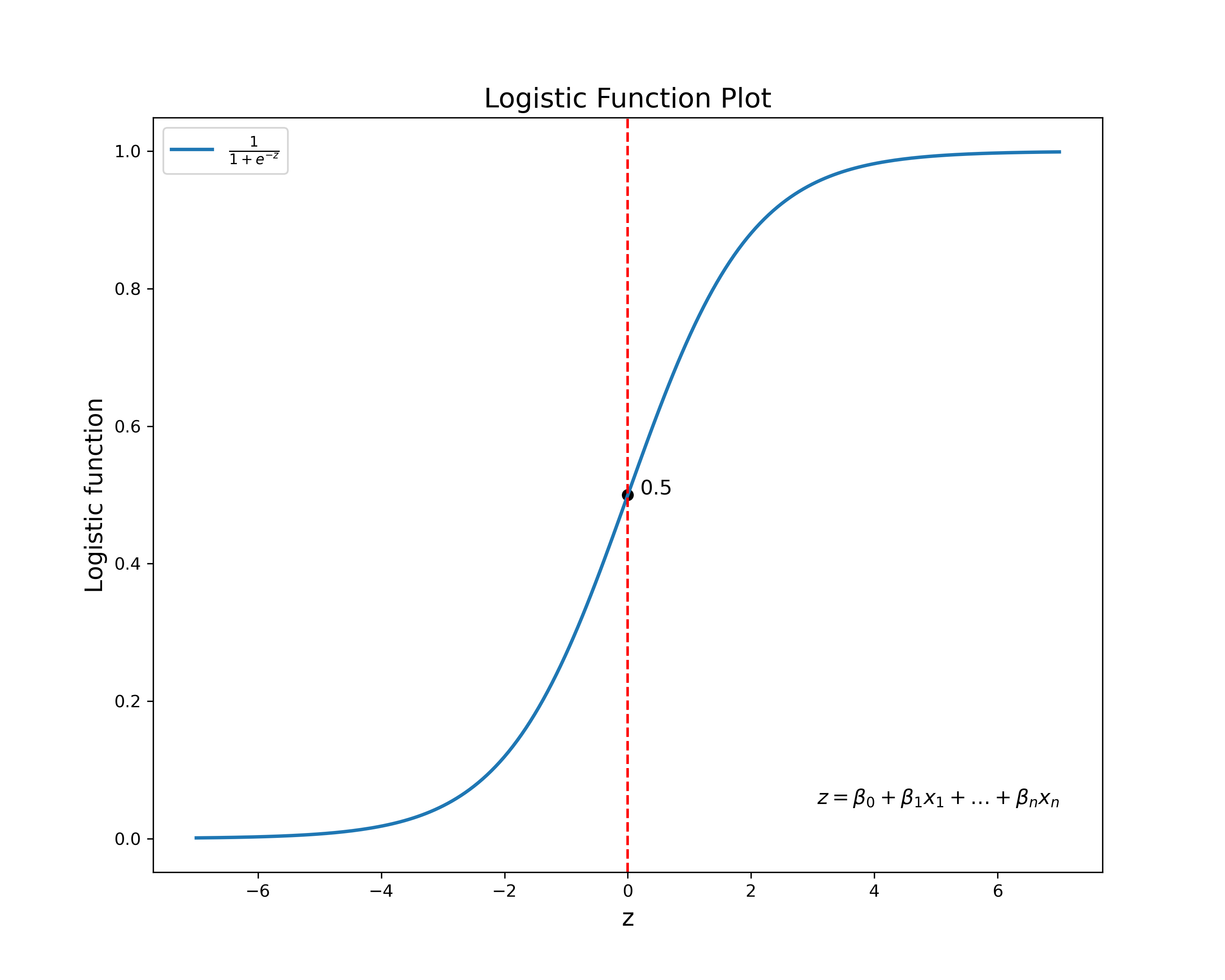
The logistic function is defined as:
$$P(Y=1 | X) = \sigma(z) = \frac{1}{1+e^{-z}}$$
Here \(z\) is defined as:
$$z = \theta_0 + \theta_1 x_1 + \theta_2 x_2+ ... \theta_n x_n = \theta^T x$$
and
\(P(Y=1 | X)\) is the probability of the outcome,
\(X = (x_1, x_2, ..., x_n)\) represents the input features variables.
\(\theta_0\) is the intercept, \(\theta_1, \theta_2, ..., \theta_n\) are the coefficients for the input features variables.
\(z\) is the linear combination of the input features.
\(\theta^T\) represents the transpose of the parameter vector.
'\(e\)' is the base of the natural logarithm (approximately equal to 2.71828).
Sometimes the logistic function is also represented in more compact form as \(h_\theta(x)\) and \(\sigma(z)\) and known as sigmoid function also known as
'activation function' (for more details, see various activation functions Optimization functions):
$$h_\theta(x) = \frac{1}{1+e^{-\theta^T x}}$$
where:
\(h_\theta(x)\) is the predicted probability that \(y = 1\).
\(\theta^T\) is the transpose of the parameter vectors
\(x\) is the input feature vector
The logistic function has an S-shaped curve (thus also known as Sigmoid function).
The logistic function maps any real-valued number to a value between 0 and 1, which can be interpreted as a probability. The goal of logistic regression is to find the values of the coefficients that maximize the likelihood of
observing the data, given the model. This is typically done using maximum likelihood estimation. Once the coefficients have been estimated, the logistic regression model can be used to predict the probability of the outcome
for new observations.
Example: For example, if we have a new observation with predictor variables \(x_1=1, x_2=3\) and \(x_3=4\), and the estimated coefficients are \(\theta_0 = -1, \theta_1 =0.5, \theta_2 = 1\) and \(\theta_3 = 0.2\),
we can calculate the probability of the outcome as follows:
$$z = -1 +0.52 +13 +0.2 \times 4 = 3.3$$
and hence,
$$P(Y = 1 | X) = \frac{1}{1+e^{-3.3}} = 0.96$$
Therefore, the probability of the outcome for this new observation is 0.96. It's important to note that logistic regression assumes a linear relationship between the predictor variables and the log odds of the outcome. This means that the logistic
regression model assumes that the relationship between the predictor variables and the probability of the outcome can be modeled using a linear equation.
From above equation, we can re write following equations:
$$\text{ln}\left(\frac{P(Y=1 | X)}{1- P(Y=1 | X)}\right) = z = \theta_0 + \theta_1 x_1 + ... + \theta_n x_n . $$
The right hand side of the equation is a linear function. Such models are called generalized linear models (GLM). In GLM, the errors may not follow normal distribution and there exists a transformation function of the outcome variable that takes a linear
functional form.
How Sigmoid function works?
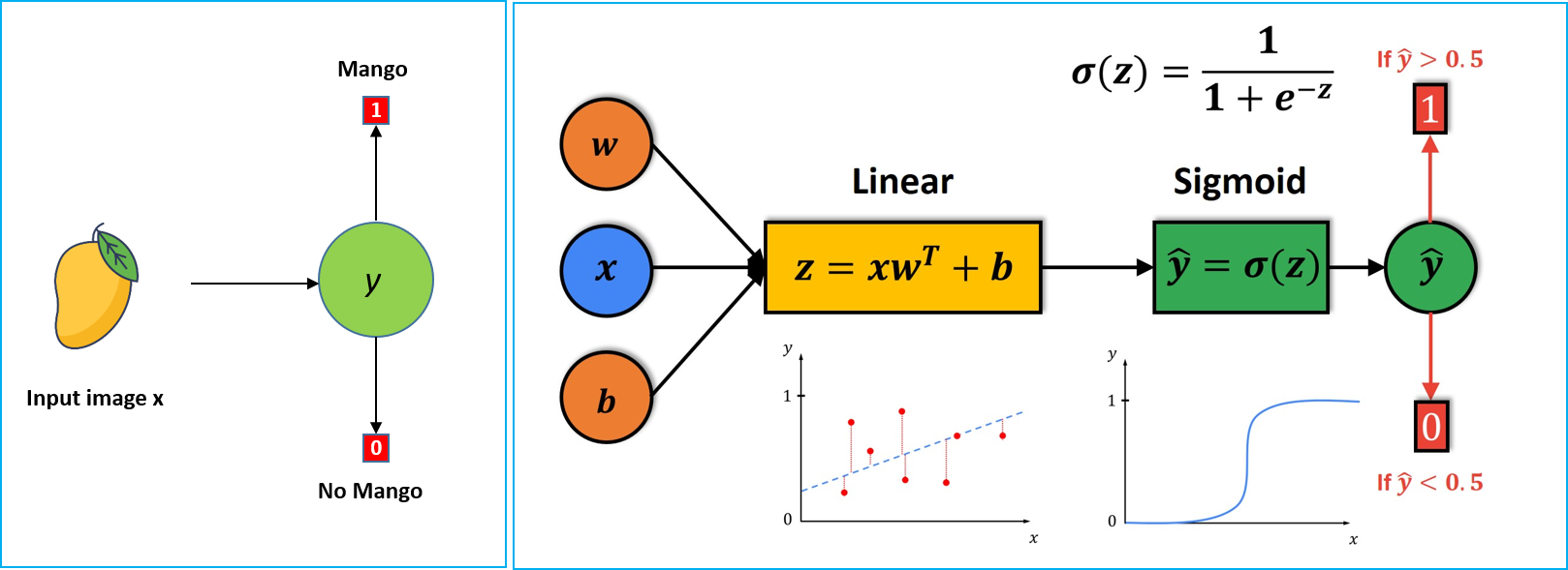
Let's say we provide an image of a fruit to our model. The model analyzes the image's features and computes a raw output score.
This raw score is then passed through the sigmoid function, which converts it into a probability score. Based on the probability outcomes generated for a given image, we determine whether the fruit in the image is a mango or not.
Here \(x\) represents out input image. \(y\) denotes the output and it can have two values, 1 or 0.if \(y=1 \), there is a mango in an image; else, if \(y=0 \), there is no mango in the image. (Image credit: Left image is credited to @ arunp77 and the
right image is taken from datahacker.rs (a nice description))
In this image, it is clear that we first calculate the output of a linear function \(z\). This output \(z\) will be the input to the Sigmoid Function.
Next, for calculated \(z \) we will produce prediction \(\hat{y} \) which will be determined by the \(z \). Then, if \(z \) is large positive value, the \(\hat{y} \) will be close to 1. On the other hand, if \(z \) is a large negative value, the \(\hat{y} \) will be close to 0. Therefore, the \(\hat{y} \) will always be in the range between 0 to 1.
One simple way to classify the prediction \(\hat{y} \) is to use a threshold value of 0.5. So, if our prediction is greater than 0.5, we assume that \(y \) is 1. Otherwise, we will assume that \(y \) is 0. As the \(\hat{y} \) gets closer to 1, the probability that there is a cat in the image becomes higher. On the other hand, as the \(\hat{y} \) comes closer to 0, the probability that there is a cat in the image also becomes lower.
To calculate the \(\hat{y} \), we will use the following equations. It is a very simple calculation wherein we will just plug in the Sigmoid Function formula into the linear model.
Linear Model:
$$\hat{y}=w^{T}x+b $$
Sigmoid Function:
$$ \sigma(z)=\frac{1}{1+e^{-z}} $$
If \(z \) is a large positive number, then:
$$\sigma (z)=\frac{1}{1+0}\approx 1 $$
If \(z \) is a large negative number, then:
$$ \sigma (z)=\frac{1}{1+\infty }\approx 0 $$
Logistic Regression Model:
$$ \hat{y}=\sigma(w^{T}x+b) $$
So, when we implement Logistic Regression, our primary goal is to attempt computing the parameters \(w \) and \(b \), such that \(\hat{y} \) becomes a good estimate of the chance of \(y=1 \). To do this, cost functions are used.
Cost function for binary Logistic Regression
Now, to train the parameters \(w \) and \(b \) of our Logistic Regression model, we need to define a Cost Function. For each data point \(x \), we start computing a series of operations to produce a predicted output.
Then, we compare this predicted output to the actual output and calculate a prediction error. This error is what we minimize during the learning process using an optimization strategy.
The way we’re computing that error value is by using a Loss Function. Our ultimate goal is to minimize the Loss Function in order to identify the values of \(w \) and \(b \). For this, we use an algorithm called the Gradient Descent.
The loss (error) function, to measure how well our algorithm is doing is defined as: \(\mathcal{L}(\hat{y}, y) = \frac{1}{2} (\hat{y} - y)^2\), (it is to be noted is that loss function is applied only to a single training sample).
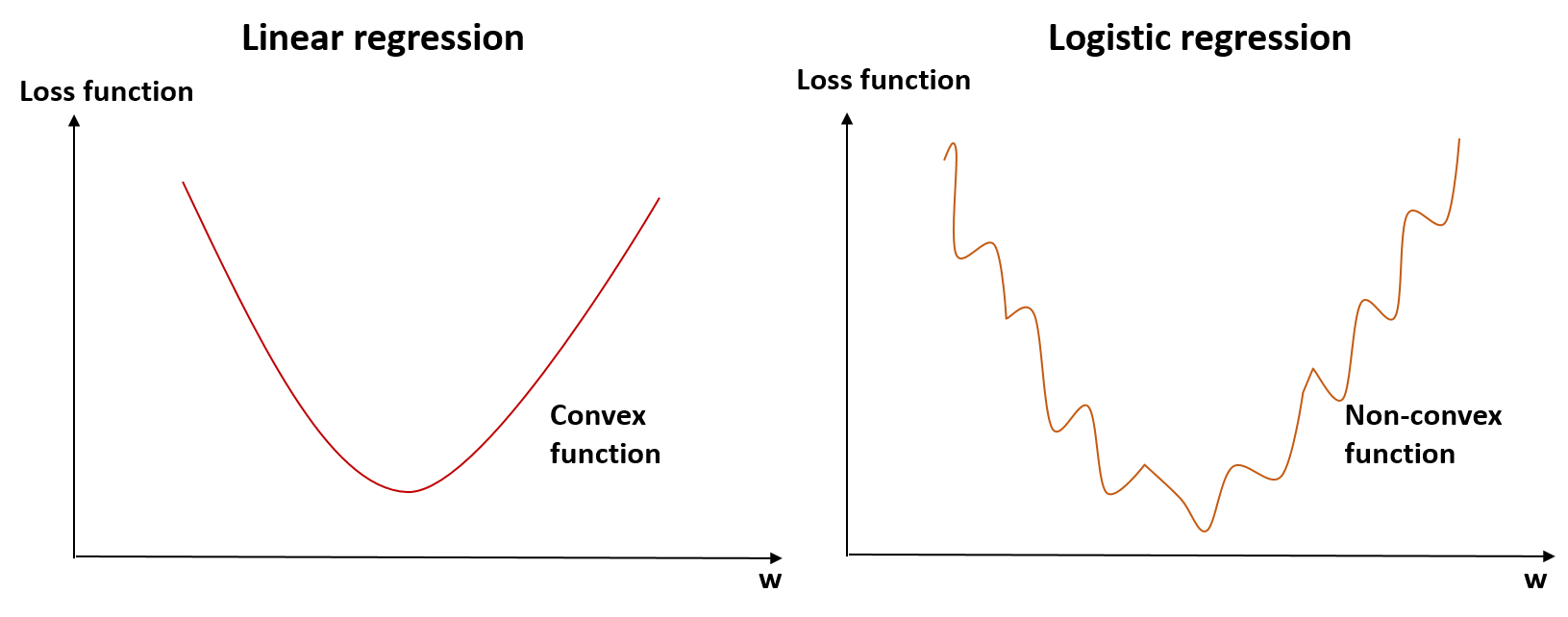
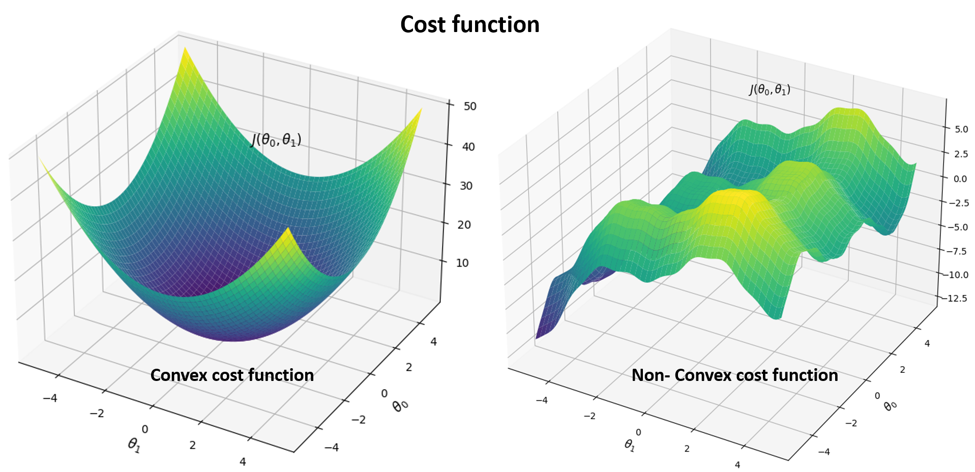
In the case of Linear regression models, a loss function is a convex function. However in the case of Logistic regression, it is a non-convex function.
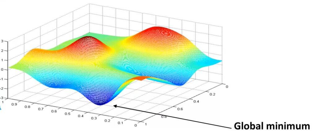
So in the case of Liear regression, GD will take steps until it converges at the global minima. However in the case of non-convex functions, there are so many local minima and hence squared error cost function is not a good choice.
Instead, there will be different cost function which makes the cost function convex again and the GD method guaranteed to converge to the global minimum. A great pictorization of the non-convex in the 3D format can be seen at the top of this page.
To ensure convergence to the global optimum, we utilize the Cross-Entropy Loss function. This metric evaluates the effectiveness of a classification model that produces probability values ranging from 0 to 1. We can write it as:
\(\mathcal{L}(\hat{y}, y) =-(y \text{log}\hat{y}+(1-y)\text{log}(1-\hat{y}))\) and hence, when \(y =1\), loss function becomes \(\mathcal{L}( \hat{y}, y) = – \text{log}\hat{y} \) should be large, so, we want \(\hat{y} \) large (as close as possible to 1 ).
However, when \(y=0\), the loss function is given by \(\mathcal{L}(\hat{y}, y) =-\text{log}(1-\hat{y})\) should be large, so, we want \(\hat{y} \) small (as close as possible to 0 ). Remember, \(\hat{y}\) is a Sigmoid Function such that it cannot be less than 0 and bigger than 1.
Now, we can define our Cost Function which measures how well our parameters \(w \) and \(b \) are doing on the entire training set. Here, we will use \((i) \) superscript to index different training examples.
\(y^{(i)}\) is the actual output for the i-th training example.
\(h_\theta (x^{(i)})\) is the predicted output for the i-th training example using the logistic function.
It is to be noted here that the Cost function \(J(\theta)\) is defined as the average of the sum of Loss functions and is a function of both weights \(\theta\) and indirectly on bias \(b\).
The cost function penalizes large errors, and the logarithmic terms ensure that the cost is higher when the prediction is far from the actual value.
For code to plot these, see code (Image credit: @ arunp77)
In training, the goal is to find the parameter vector \(\theta\) that minimizes the cost function. This is often done using optimization algorithms like gradient descent or Maximum Likelihood Estimation (MLE) method.
Multi-Class Logistic Cost function
Let's delve into the mathematical formulations of both the One-vs-Rest (OvR) and Multinomial Logistic Regression approaches:
One-vs-Rest (OvR) Logistic Regression:
Let us assume a scenario for each class \(k\) in a multi-class classification problem with \(K\) classes.
Assume that we have a set of features \(x\) and parameters \(\theta^{(k)}\) for each class \(k\).
The hypothesis function \(h_\theta^{(k)}(x)\) represents the probability that example \(x\) belongs to class \(k\).
The hypothesis function is given by the sigmoid (logistic) function:
$$h_{\theta}^{(k)}(x) = \frac{1}{1+e^{-\theta^{(k)T}x}}.$$
We train \(K\) separate logistic regression models, each predicting the probability of one class vs. all other classes.
For class \(k\), the cost function is the binary cross-entropy loss:
$$J(\theta^{(k)})= -\frac{1}{m}\sum_{i=1}^{m} \left[ y^{(i)} \text{log}(h_{\theta}^{(k)}(x^{(i)}))+(1-y^{(i)})\text{log}(1-h_\theta^{(k)}(x^{(i)}))\right]$$
where, \(y^{(i)}\) is the binary indicator (0 or 1) if example \(i\) belongs to class \(k\).
To predict the class for a new example \(x\), we compute the probabilities \(h_\theta^{(k)}(x)\) for each class \(k\), and select the class with the highest probability.
Multinomial Logistic Regression (Softmax Regression):
Consider a multi-class classification problem with \(K\) classes.
We have a set of feature \(x\) and parameters \(\Theta\), where \(\Theta\) is a matrix of size \((n\times K)\) for \(n\) features and \(K\) classes.
The hypothesis function \(h_\Theta(x)\) outputs a probability distribution over all \(K\) classes.
The softmax function computes the probability of each class:
Here, \(h_\Theta(x)_k\) is the probability that example \(x\) belongs to class \(k\).
The cost function is the categorical cross-entropy loss, also known as the softmax loss:
$$J(\Theta) = -\frac{1}{m} \sum_{i=1}^m \sum_{k=1}^K y_k^{(i)} \text{log}(h_\Theta(x^{(i)})_k)$$
where, \(y_k^{(i)}\) is the binary indicator (0 or 1) if example \(i\) belongs to class \(k\).
To predict the class for a new example \(x\), we compute the probabilities \(h_\Theta(x)\) for all \(K\) classes, and select the class with the highest probability.
Gradient Descent Rule:
The gradient descent algorithm for the logistic regression aims to find the optimal parameters \(\theta\) and \(w\)
that minimize the cost function. The update rule is derived from the partial derivatives of the cost function with respect to each parameter.
The update rule for the gradient descent algorithm is as follows:
Maximum Likelihood Estimation (MLE) is a statistical method used to calculate the parameters. In the case of logistic regression, MLE aims to find the set of parameters that maximizes the likelihood function, which measures how well the model explains the observed data.
Mathematical Description:
For logistic regression, let's denote the likelihood function as \(L(\theta)\), where \(\theta\) represents the parameters of the logistic regression model. The likelihood function is given by the product of the
probabilities of the observed outcomes under the current parameter values.
For a binary classification problem (0 or 1), the likelihood function is often expressed as:
\(y^{(i)}\) is the actual output for the i-th training example (0 or 1).
\(x^{(i)}\) is the input feature vector for the i-th training example.
\(P(y^{(i)|x^{(i); \theta}})\) is the predicted probabolity if the i-th example belonging to class 1.
In logistic regression, the predicted probability is given by the logistic function:
$$P(y^{(i)} =1| x^{(i)}; \theta) = h_\theta(x^{(i)})$$
$$P(y^{(i)} =0| x^{(i)}; \theta) = 1- h_\theta(x^{(i)})$$
The goal of MLE is to find the values of \(\theta\) that maximize the likelihood function \(L(\theta)\). In practice, it
is often more convenient to maximize the log-likelihood function (logarithm of the likelihood function), denoted as \(l(\theta)\):
$$l(\theta) = \sum_{i=1}^m \left[y^{(i)} \text{log}(h_\theta(x^{(i)}))- (1-y^{(i)})\text{log}(1-h_\theta(x^{(i)}))\right].$$
Maximizing \(l(\theta)\) is equivalent to maximizing \(L(\theta)\), as the logrithm is a monotonically increasing function.
The logistic regression cost function \(J(\theta)\) that we discussed earlier is essentially the negative log-likelihood, with some scaling for convenience in optimization:
$$J(\theta) = -\frac{1}{m} l(\theta).$$
So, in logistic regression, the optimization process, whether using gradient descent or another optimization algorithm, is essentially performing Maximum Likelihood Estimation to find the parameters that maximize the likelihood of observing the given set of training examples.
Confusion matrix
The confusion matrix is a tool used in classification to evaluate the performance of a machine learning model. It is a matrix of actual classes vs. predicted classes. Here's the formula to compute it:
Let's assume we have a binary classification problem with two classes: Positive (P) and Negative (N).
True Positive (TP): The model correctly predicts positive instances.
True Negative (TN): The model correctly predicts negative instances.
False Positive (FP): The model incorrectly predicts positive instances as negative.
False Negative (FN): The model incorrectly predicts negative instances as positive.
The confusion matrix is typically represented as:
Confusion matrix (Image credit: @ arunp77)
Lets learn about few metrics that help in understanding how well the model is performing in terms of correctly and incorrectly classifying instances.
Accuracy:Accuracy is a common metric used to evaluate the performance of a classification model. It represents the ratio of correctly predicted instances to the total instances in the dataset. Mathematically, accuracy is calculated as:
$$\text{Accuracy} = \frac{\text{Number of Correct Predictions}}{\text{Total number of predictions}} = \frac{\text{TP+TN}}{\text{TP+TN+FP+FN}}.$$
A higher accuracy value indicates better performance of the model in making correct predictions across all classes. However, accuracy alone might not provide a complete picture of the model's performance, especially in scenarios where classes are imbalanced or have different costs associated with misclassification. Therefore, it's essential to consider other evaluation metrics along with accuracy.
Precision, recall & F-score: Precision and recall are two important metrics used to evaluate the performance of a classification model, especially in scenarios where class imbalance exists.
Precision: Precision measures the accuracy of positive predictions made by the model. It is the ratio of true positive predictions to the total number of positive predictions made by the model.
Mathematically, it is defined as:
$$\text{Precision} = \frac{\text{TP}}{\text{TP+FP}}$$
Precision answers the question: "Of all the instances predicted as positive, how many are actually positive?" A high precision indicates that the model is making fewer false positive predictions.
Recall (Sensitivity):Recall, also known as sensitivity or true positive rate, measures the model's ability to correctly identify positive instances. It is the ratio of true positive predictions to the total number of actual positive instances in the dataset.
Mathematically, recall is calculated as:
$$\text{Recall} = \frac{\text{TP}}{\text{TP+FN}}.$$
Recall answers the question: "Of all the actual positive instances, how many did the model correctly predict as positive?" A high recall indicates that the model is effectively capturing most of the positive instances.
Both precision and recall are important metrics, and there is often a trade-off between them. For example, increasing precision may lead to a decrease in recall and vice versa. The F1 score, which is the harmonic mean of precision and recall, is often used to balance these two metrics.
F-score: The F-score, also known as the F1 score, is a single metric that combines precision and recall into a single value. It provides a balance between precision and recall, considering both false positives and false negatives.
Mathematically, the F1 score is the harmonic mean of precision and recall and is calculated as:
$$F_\beta = (1+\beta^2)\times \frac{\text{Precision} \times \text{Recall}}{(\beta^2\times \text{Precision})+\text{Recall}}.$$
where
\(\beta =1\), then \(F_1 = 2 \times \frac{\text{Precision} \times \text{Recall}}{\text{Precision}+\text{Recall}}\). It is known as harmonic mean. It equally weights precision and recall, making it suitable when both false positives and false negatives have similar costs or when there is no significant preference between precision and recall.
The F1 score reaches its best value at 1 (perfect precision and recall) and worst at 0. It provides a single value that summarizes the performance of a classification model, especially in scenarios where class imbalance exists or when both precision and recall are equally important.
\(\beta =2\), then \(F_2 = 5 \times \frac{\text{Precision} \times \text{Recall}}{4\times \text{Precision}+\text{Recall}}\). It gives more weight to recall than precision, making it suitable for tasks where recall is more critical than precision. For example, in medical diagnostics, where missing a positive case (low recall) might have more severe consequences than a false alarm (low precision).
\(\beta =0.5\), then \(F_{0.5} = \frac{1.25 \times \text{Precision} \times \text{Recall}}{0.25\times \text{Precision}+\text{Recall}}\). It gives more weight to precision than recall, making it suitable for tasks where precision is more critical than recall. For example, in spam detection, where it's crucial to minimize false positives (high precision) even if it means missing some spam emails (low recall).
\(\beta =1\), then \(F_1 = 2 \times \frac{\text{Precision} \times \text{Recall}}{\text{Precision}+\text{Recall}}\).
Example project
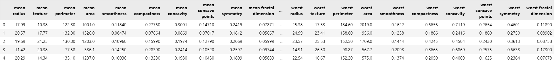
The load_breast_cancer dataset is a built-in dataset in scikit-learn that contains features computed from a digitized image of a fine needle aspirate (FNA) of a breast mass. The dataset is used for binary classification tasks, particularly for distinguishing between malignant and benign tumors. Here are some details about the dataset:
Features: The dataset consists of 30 features computed from images of FNA of breast masses. These features represent various characteristics of the cell nuclei present in the images, such as radius, texture, smoothness, compactness, concavity, symmetry, fractal dimension, etc.
Target: The target variable represents the diagnosis of the tumor. It is binary, with 0 indicating a malignant (cancerous) tumor and 1 indicating a benign (non-cancerous) tumor.
Size: The dataset contains a total of 569 instances (samples), with each instance having 30 features and a corresponding target label.
            from sklearn.linear_model import LogisticRegression
            from sklearn.datasets import load_breast_cancer

            df = load_breast_cancer()

            # Independent features
            X = pd.DataFrame(df['data'], columns=df['feature_names'])
            # Depednent feature
            y = pd.DataFrame(df['target'], columns=["Target"])
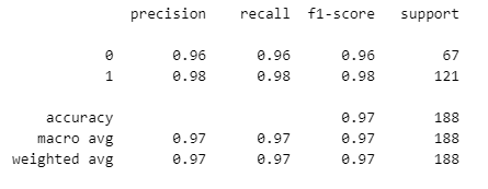
Precision: Precision is the ratio of correctly predicted positive observations to the total predicted positives. In other words, it measures the accuracy of positive predictions. For class 0, precision is 0.96, and for class 1, precision is 0.98. This indicates that the model performs well in predicting both classes, with slightly higher precision for class 1.
Recall (Sensitivity): Recall is the ratio of correctly predicted positive observations to the all observations in the actual class. It measures the ability of the classifier to find all the positive samples. For class 0, recall is 0.96, and for class 1, recall is 0.98. This indicates that the model effectively identifies both classes, with slightly higher recall for class 1.
F1-score: The F1-score is the harmonic mean of precision and recall. It provides a balance between precision and recall. For class 0, the F1-score is 0.96, and for class 1, the F1-score is 0.98. This indicates a good balance between precision and recall for both classes.
Support: Support is the number of actual occurrences of the class in the specified dataset. For class 0, the support is 67, and for class 1, the support is 121.
Accuracy: Accuracy is the ratio of correctly predicted observations to the total observations. It measures the overall correctness of the model. In this case, the accuracy is 0.97, indicating that the model correctly predicts 97% of the observations in the dataset.
Macro Avg: The macro average calculates the average metric (precision, recall, F1-score) across all classes. In this case, the macro average precision, recall, and F1-score are all 0.97, indicating good overall performance across classes.
Weighted Avg: The weighted average calculates the average metric (precision, recall, F1-score) across all classes, weighted by the number of true instances for each class. In this case, the weighted average precision, recall, and F1-score are all 0.97, indicating good overall performance considering the class imbalance.
You can go to following project for a reference for linear regression analysis.