
The Role and Importance of Optimization in Deep Learning
Introduction
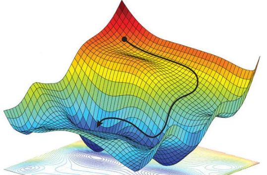
Optimization lies at the heart of deep learning, playing a crucial role in training neural networks to achieve high performance on various tasks such as image classification, natural language processing, and reinforcement learning. By iteratively adjusting the parameters of a neural network, optimization algorithms seek to minimize a predefined objective function, often referred to as the loss or cost function.This process involves finding the optimal set of parameters that result in the best possible model performance.
Below, I will discuss the role and importance of optimization techniques in deep learning.
Optimization in deep learning is vital for several reasons:
- Model Convergence: Effective optimization ensures that the training process converges to a set of parameters where the model exhibits satisfactory performance on unseen data.
- Enhanced Performance: Well-optimized models tend to achieve higher accuracy, better generalization, and faster convergence during training.
- Scalability: Optimization algorithms need to scale efficiently to handle large datasets and complex neural network architectures commonly encountered in deep learning tasks.
- Robustness: Robust optimization methods help neural networks avoid overfitting and learn meaningful representations from data, leading to improved performance on diverse tasks.
Optimization at work
Optimization algorithms iteratively update model weights to minimize the loss function. Here's a simplified description of the process:- Forward Pass: Data flows through the network, generating predictions.
- Loss Calculation: The loss function compares the predictions against desired outputs, measuring error.
- Backpropagation: The error signals are propagated back through the network, calculating "gradients" that indicate how weights should change to reduce the loss.
- Weight Update: The optimizer (e.g., gradient descent, Adam) uses the gradients to update the network's weights.
Optimization Methods in Deep Learning
In deep learning, optimizers are crucial as algorithms that dynamically fine-tune a model’s parameters throughout the training process, aiming to minimize a predefined loss function. These specialized algorithms facilitate the learning process of neural networks by iteratively refining the weights and biases based on the feedback received from the data. Well-known optimizers in deep learning encompass Stochastic Gradient Descent (SGD), Adam, and RMSprop, each equipped with distinct update rules, learning rates, and momentum strategies, all geared towards the overarching goal of discovering and converging upon optimal model parameters, thereby enhancing overall performance.
Optimizers: During the training of deep learning models, optimizers play a crucial role by adjusting parameters like weights and learning rates to minimize the loss function and enhance accuracy. As deep learning models typically contain millions of parameters, selecting the right optimizer is a challenging task. Understanding various optimization algorithms is essential for data scientists to effectively navigate the field. Different optimizers can be employed in machine learning models to alter weights and learning rates. However, the choice of the best optimizer depends on the specific application. While it may seem tempting for beginners to experiment with various optimizers and select the one yielding the best results, this approach becomes impractical when dealing with large datasets. Randomly selecting an optimizer can lead to significant time wastage, akin to gambling with valuable resources. Therefore, it's crucial to make informed decisions when choosing optimizers to avoid unnecessary delays and optimize training efficiency.
Terminologies
- Model: A mathematical function that transforms inputs into outputs, incorporating a set of adjustable parameters and an accompanying algorithm for optimization.
- Model Parameter: A tunable element within a neural network, utilized to refine the accuracy and efficiency of the model. Common instances include weights and biases in a feedforward neural network, which are adjusted during training to optimize performance.
- Epoch: The number of times the algorithm runs on the whole training dataset.
- Sample: A single row of a dataset
- Batch: It denotes the number of samples to be taken to for updating the model parameters.
- Learning rate: It is a parameter that provides the model a scale of how much model weights should be updated.
- Cost function/Loss function: A cost function is used to calculate the cost, which is the difference between the predicted value and the actual value.
- Weights/bias: The learnable parameters in a model that controls the signal between two neurons.
Now let’s explore each optimizer.
1. Gradient Descent (GD):
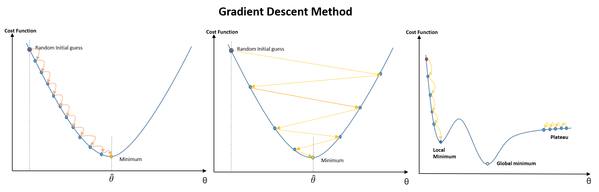
- Objective: Gradient Descent is an iterative optimization algorithm used to minimize a given cost function \(J(\theta)\) by adjusting the parameters \(\theta\) iteratively.
- Components:
- Cost Function (Loss Function): \(J(\theta_t)\) represents the cost function or loss function that measures how well the model performs on the training data with respect to its parameters \(\theta\).
- Gradient: The gradient of the cost function \(J(\theta)\) with respect to the parameters \(\theta\), denoted by \(\nabla J(\theta)\), represents the direction of the steepest ascent. The negative gradient \(-\nabla J(\theta)\) points in the direction of the steepest descent, i.e., the direction in which the function decreases most rapidly.
- Learning rate (\(\eta\)): \(\eta\) is a hyperparameter known as the learning rate. It determines the size of the steps taken in the parameter space during each iteration of the optimization process.
- Steps:
- Initialization: Initialize the parameters \(\theta\) randomly or with certain pre-defined values.
- Compute Gradient: Calculate the gradient of the cost function \(J(\theta)\) with respect to the parameters \(\theta\) at the current parameter values
- Update Parameters: Update the parameters \(\theta\) in the opposite direction of the gradient by taking a step proportional to the
negative gradient and the learning rate. This step is expressed by the formula:
$$\theta_{t+1} = \theta_t - \eta \nabla J(\theta_t)$$
where
- \(\theta_{t+1}\) is the updated value of parameters at iteration \(t+1\).
- \(\theta_t\) is the current value of parameters at iteration \(t\).
- \(\nabla J(\theta_t)\) is the
- \(\eta\) is the learning rate
- Repeat
- Convergence: Convergence occurs when the algorithm reaches a point where further updates to the parameters do not significantly reduce the value of the cost function.
- Summary: Gradient Descent iteratively updates the parameters \(\theta\) in the direction of the steepest descent of the cost function, aiming to minimize the cost function and thereby optimize the model.
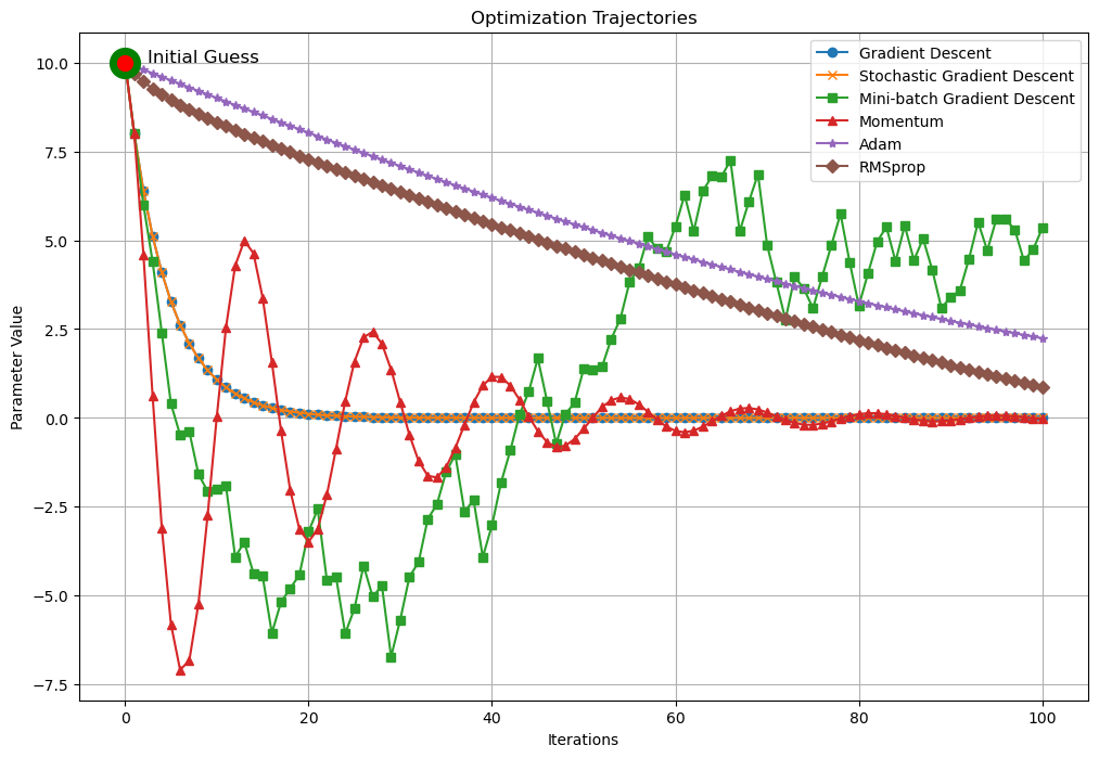
- Variants: Various variants of Gradient Descent, such as Stochastic Gradient Descent (SGD), Mini-batch Gradient Descent, Momentum, Adam, and RMSprop, introduce modifications to the basic algorithm to improve convergence speed, stability, and efficiency.
2. Stochastic Gradient Descent (SGD):
- Objective: SGD is an optimization algorithm commonly used in machine learning and deep learning for training models. It aims to minimize a given loss function by iteratively updating the model parameters.
- Basic Idea:: Instead of computing the gradient of the loss function over the entire dataset (as in batch gradient descent), SGD computes the gradient over a single random training example at each iteration.
- Algorithm:
- Initialization: Start with initial parameter values \(\theta_0\).
- Loop: Repeat until convergence or for a fixed number of iterations:
- Randomly shuffle the training dataset.
- For each training example \(i\) in the dataset:
- Compute the gradient of the loss function with respect to the parameters using the current example: \(\nabla J(\theta_{t, i})\).
- Update the parameters using the gradient descent update rule: $$\theta_{t+1} = \theta_t - \eta \nabla J(\theta_{t,i})$$ where:
- \(\theta_t\) is the parameter vector at iteration \(t\).
- \(\eta\) is the learning rate, determining the step size.
- Key Aspects:
- Randomness: SGD introduces randomness by using a random training example at each iteration. This randomness helps escape local minima and can lead to faster convergence, especially in large datasets.
- Efficiency: Since only one training example is processed per iteration, SGD is computationally efficient and can handle large datasets that may not fit into memory.
- Noisy Updates: Due to the randomness, SGD updates can be noisy, leading to oscillations around the optimal solution. However, this noise can sometimes help the optimization process by escaping sharp local minima.
- Learning Rate Tuning: The learning rate \(\eta\) plays a crucial role in SGD. Choosing an appropriate learning rate is essential for convergence. It may need to be tuned during training using techniques like learning rate schedules or adaptive learning rate methods.
- Formula: The update rule for SGD using a single training example \(i\) can be represented as:
$$\theta_{t+1} = \theta_{t} - \eta \nabla J(\theta_{t,i})$$
where:
- \(\theta_t\) is the parameter vector at iteration \(t\).
- \(\eta\) is the learning rate.
- \(\nabla J(\theta_{t,i})\) is the gradient of the loss function with respect to the parameters computed using the \(i-\)th training example.
- Advantages:
- Efficiency: SGD is computationally efficient, making it suitable for large-scale datasets.
- Generalization: It often leads to better generalization since it avoids overfitting by updating parameters frequently with different examples.
- Parallelism: SGD is inherently parallelizable, allowing for efficient implementation on parallel computing architectures.
- Disadvantages:
- Noisy Updates: The randomness in SGD updates can lead to noisy convergence, making it challenging to find the exact optimal solution.
- Learning Rate Tuning: Proper tuning of the learning rate is crucial for stable convergence. An inappropriate learning rate can lead to slow convergence or divergence.
- Sensitive to Scaling: SGD can be sensitive to feature scaling, requiring careful preprocessing of the input data.
3. Mini-batch Gradient Descent:
Mini-batch Gradient Descent (MBGD) is a variation of the traditional Gradient Descent algorithm that updates the model parameters using mini-batches of training data instead of the entire dataset at once. This approach combines the efficiency of Stochastic Gradient Descent (SGD) with the stability of Gradient Descent (GD). Here's a detailed explanation of MBGD along with the relevant formulas:- Overview: Mini-batch Gradient Descent divides the training data into small batches of size \(n\). Instead of computing the gradient on the entire dataset (GD) on on a single data point (SGD), MBGD computes the gradient on a mini-batch of training examples.
- Formulation: Let's consider a dataset with \(m\) training examples. The cost function \(J(\theta)\) measures the difference between the model predictions and the actual targets. The update rule for Mini-batch Gradient Descent at iteration \(t\) is given by: $$\theta_{t+1} = \theta_t - \eta \nabla J(\theta_{t,i:i+n})$$ where:
- \(\theta_t\) is the parameter vector at iteration \(t\).
- \(\eta\) is the learning rate.
- \(\nabla J(\theta_{t,i:i+n})\) is the gradient of the cost function \(j(\theta)\) computed on the mini-batch \(i:i+n\).
- Algorithm Steps:
- Initialization: Initialize the model parameters \(\theta\) and hyperparameters like the learning rate \(\eta\).
- Mini-batch Formation: Randomly shuffle the training data and divide it into mini-batches of size \(n\). If the dataset size is not divisible by \(n\), the last mini-batch may have fewer examples.
- Gradient Computation: For each mini-batch \(i : i+n\), compute the gradient of the cost function \(J(\theta)\) with respect to the parameters \(\theta\): $$\nabla J(\theta_{t,i:i+n}) = \frac{1}{n} \sum_{j=i}^{i+n} \nabla J(\theta_{t},x_j, y_j)$$ where (\(x_j,y_j\)) are the input features and corresponding target labels in the min-batch.
- Parameter Update: Update the parameter \(\theta\) using the computed gradient: $$\theta_{t+1} = \theta_t - \eta \nabla J(\theta_{t,i:i+n})$$
- Repeat: Repeat steps (c) and (d) for a fixed number of iterations or until convergence criteria are met.
- Benefits of Mini-batch Gradient Descent:
- Efficiency: MBGD utilizes vectorized operations, making it computationally efficient compared to SGD.
- Stability: It offers more stable convergence than SGD as it considers a mini-batch of examples.
- Memory Usage: It allows for efficient memory usage by processing only a subset of data at a time.
- Hyperparameter Tuning:
- Batch Size \(n\): The choice of mini-batch size affects the convergence speed and memory requirements.
- Learning Rate \(\eta\): The learning rate determines the step size during parameter updates and impacts convergence.
4. Momentum:
Momentum is an optimization technique that helps accelerate gradient descent algorithms in the relevant direction and dampens oscillations. It accomplishes this by adding a fraction of the previous update vector to the current gradient. This helps to smooth out the steps taken during optimization, especially when the cost surface has high curvature or noisy gradients.Here's a detailed explanation of Momentum along with the formulas involved:
- Update Formulas:
- Momentum introduces a variable \(v\) which accumulates the gradients of the past steps.
- The update for \(v\) at each iteration \(t\) is given by: $$v_{t+1}= \beta v_t + (1-\beta) \nabla J(\theta_t)$$ where:
- \(v_t\) is the momentum at time step \(t\),
- \(\nabla J(\theta_t)\) is the gradient of the cost function \(J\) with respect to the parameters \(\theta\) at time step \(t\),
- \(\beta\) is the momentum parameter, typically set to a value close to 1, e.g., 0.9.
- Then, the parameter \(\theta\) are updated using the momentum term: $$\theta_{t+1} = \theta_t - \eta v_{t+1}$$ where \(\eta\) is the learning rate.
- Explanation of Formulas:
- The first term in the update equation for \(v\) is the momentum term (\(\beta v_t\)), which is the previous momentum scaled by the momentum parameter \(\beta\).
- The second term in the update equation is the gradient of the cost function scaled by (1-\(\beta\)), which gives the contribution of the current gradient.
- The momentum term effectively remembers the direction of previous gradients and reinforces the current direction if gradients keep pointing in the same direction, thus helping to speed up convergence.
- If the gradients keep changing direction (e.g., during oscillations), the momentum term helps to smooth out these oscillations by accumulating gradients in a consistent direction.
- Advantages of Momentum:
- Helps accelerate convergence, especially in the presence of high curvature or noisy gradients.
- Dampens oscillations and overshooting in the optimization process, leading to more stable and efficient training.
- Helps to escape local minima or saddle points by accumulating momentum to push through flat regions.
- Choosing the Momentum Parameter \(\beta\):
- The momentum parameter \(\beta\) typically ranges from 0.8 to 0.999.
- A higher value of \(\beta\) takes the algorithm more "momentum-heavy," which can help in smoothing our oscillations but might overshoot minima.
- A lower value of \(\beta\) makes the algorithm more responsive to recent gradients but might slow down convergence.
5. Adam (Adaptive Moment Estimation):
Adam (Adaptive Moment Estimation) is an optimization algorithm commonly used in deep learning, known for its adaptive learning rate and momentum properties. It combines the advantages of two other popular optimization algorithms, RMSprop and Momentum, to efficiently navigate the parameter space during training. Let's delve into the details of Adam and explain its various components using formulas:Algorithm Overview:
- Initialization: First Initialize parameters:
- \(\theta_0\): Model parameters (weights and biases).
- \(m_0\) = 0: Initial first moment vector (mean),
- \(v_0\) =0: Initial second moment vector (uncentered variance).
- \(\beta_1, \beta_2 \in [0,1)\): Exponential decay rates for moment estimates.
- \(\eta\): Learning rate.
- \(\epsilon\): small constant to prevent division by zero. Defaults to 1e-8.
- Update at each time step \(t\):
- Compute gradient: $$g_t = \nabla J(\theta_t)$$ where \(J\) is the loss function.
- Update biased first moment estimate: $$m_t = \beta_1\cdot m_{t-1} +(1-\beta_1)\cdot g_t$$
- Update biased second raw moment estimate: $$v_t = \beta_2 \cdot v_{t-1} + (1-\beta_2)\cdot g_t^2$$
- Correct bias in first moment: $$\hat{m}_t = \frac{m_t}{1-\beta_1^t}.$$
- Correct bias in second moment: $$\hat{v}_t = \frac{v_t}{1-\beta_2^t}$$
- Update parameters: $$\theta_{t+1} = \theta_t - \eta\cdot \frac{\hat{m}_t}{\sqrt{\hat{v}_t}+\epsilon} $$
Detailed Explanation of Formulas:
- First Moment Estimation (Mean): $$m_t = \beta_1 \cdot m_{t-1} +(1-\beta_1)\cdot g_t$$ where:
- \(m_t\): Biased first moment estimate (mean of gradients)
- \(\beta_1\): Exponential decay rate for the first moment.
- \(g_t\): Gradient at time step.
- Second Moment Estimation (Uncentered Variance): $$v_t = \beta_2 \cdot v_{t-1}+(1-\beta_2)\cdot g_t^2$$ where:
- \(v_t\): Biased second raw moment estimate (uncentered variance of gradients).
- \(\beta_2\): Exponential decay rate for the second moment.
- \(g_t^2\): Element-wise square of the gradient at time step \(t\).
- Bias Correction: $$\hat{m}_t = \frac{m_t}{1-\beta_1^t}$$ and $$\hat{v}_t = \frac{v_t}{1-\beta_2^t}.$$ where:
- Corrects bias in the first and second moment estimates, especially during the initial time steps when \(m_t\) and \(v_t\) are biased towards zero.
- Parameter Update: $$\theta_{t+1} = \theta_t -\eta \cdot \frac{\hat{m}_t}{\sqrt{\hat{v}_t}+\epsilon}.$$ where:
- Corrects bias in the first and second moment estimates, especially during the initial time steps when \(m_t\) and \(v_t\) are biased towards zero.
- Parameter Update: $$\theta_{t+1} = \theta_t - \eta\cdot \frac{\hat{m}_t}{\sqrt{\hat{v}_t}+\epsilon}.$$
- Updates the model parameters using the corrected first and second moment estimates.
- \(\eta\): Learning rate.
- \(\epsilon\): Small constant to prevent division by zero.
Key Features:
- Adaptive Learning Rate: The learning rate is adjusted for each parameter based on the estimates of the first and second moments of the gradients.
- Bias Correction: Adam corrects the bias in the moment estimates, especially at the beginning of training.
- Momentum: The first moment term \(m_t\) acts like a momentum term, allowing the algorithm to accelerate in the relevant direction and dampen oscillations.
- Efficiency: Adam is computationally efficient and requires little memory.
6. RMSprop (Root Mean Square Propagation):
RMSprop (Root Mean Square Propagation) is an optimization algorithm commonly used in deep learning to adaptively adjust the learning rates for each parameter. It addresses some of the limitations of other optimization algorithms, particularly when dealing with sparse data and non-stationary objectives. Here's a detailed explanation of RMSprop along with formulas:Overview: RMSprop is an extension of the gradient descent optimization algorithm that aims to improve convergence speed and stability, especially in the presence of sparse gradients or noisy data. It accomplishes this by adjusting the learning rates of each parameter individually based on the magnitude of recent gradients.
Algorithm Steps:
- Initialize Parameters: Initialize model parameters \(\theta\), typically randomly or using pre-trained values. Initialize a decay rate \(\beta\), usually close to 1, and a small constant \(\epsilon\) for numerical stability.
- Initialize Variables: Initialize an accumulation variable \(v\) to store the exponentially weighted moving average (EWMA) of squared gradients.
- Compute Gradients: Compute the gradients of the loss function with respect to the parameters \(\nabla J(\theta)\) using backpropagation.
- Update Accumulation: Update the accumulation variable \(v\) by taking an EWMA of the squared gradients: $$v = \beta v+(1-\beta)(\nabla J(\theta))^2$$ where \(\beta\) is the decay rate \((\nabla J(\theta))^2\) represents element-wise squaring of the gradients.
- Update Parameters: Update the parameters \(\theta\) using the RMSprop update rule: $$\theta = \theta - \eta \frac{\nabla J(\theta)}{\sqrt{v}+\epsilon}$$ where \(\eta\) is the learning rate and \(\epsilon\) is a small constant added for numerical stability to avoid division by zero.
Detailed Explanation:
- Accumulation of Squared Gradients \(v\): RMSprop maintains an exponentially decaying average of squared gradients using the parameter \(\beta\). This moving average helps smooth out the gradient updates and adaptively adjust the learning rates.
- Normalization of Gradients: Before updating the parameters, RMSprop normalizes the gradients by dividing them by the square root of the accumulated squared gradients plus a small constant \(\epsilon\). This Normalization scales down the learning rates for parameters with large gradients and vice versa.
- Adaptive Learning Rates: By adjusting the learning rates based on the magnitude of gradients, RMSprop adapts to the geometry of the loss function and speeds up convergence, especially in deep neural networks with complex and non-convex surfaces.
Key Advantages:
- Adaptive Learning Rates: RMSprop adapts the learning rates for each parameter individually based on the recent gradient history, leading to faster convergence and improved stability.
- Sparse Data Handling: The algorithm performs well with sparse data or noisy gradients, thanks to its adaptive nature and normalization of gradients.
- Robustness: RMSprop is robust to variations in hyperparameters and works well across different architectures and datasets.
Summary:
RMSprop is a powerful optimization algorithm widely used in training deep neural networks. By adaptively adjusting learning rates based on the magnitude of gradients, it addresses some of the challenges faced by traditional gradient descent methods, leading to faster convergence and improved performance.References
- “Deep Learning”: Optimization Techniques.
- Deep learning architectures
- Hands on Machine Learning with Scikit-Learn, Keras, & TensorFlow, Aurelien Geron
Some other interesting things to know:
- Look at my Deep Learning page.
- Visit my website on For Data, Big Data, Data-modeling, Datawarehouse, SQL, cloud-compute.
- Visit my website on Data engineering