Naive Bayes: Classification methods
Introduction
Naive Bayes algorithms are a family of probabilistic classifiers based on Bayes' theorem with the "naive" assumption of independence between features. Despite their simplicity, they are powerful and widely used for classification tasks in various fields, including text classification, spam filtering, and medical diagnosis. They work by calculating the probability of a given data point belonging to each class and selecting the class with the highest probability.
Naive Bayes algorithms are efficient, particularly for large datasets, and they perform well even with limited training data. Popular variants include Gaussian Naive Bayes, Multinomial Naive Bayes, and Bernoulli Naive Bayes.
Principle of Naive Bayes
At the core of Naive Bayes is Bayes' theorem, which calculates the probability of a hypothesis (class label) given the observed evidence (features). The "naive" assumption in Naive Bayes is that the features are conditionally independent given the class label, which simplifies the calculation of probabilities.
- \(P(A|B)\) is the probability of event \(A\) occurring given that event \(B\) has occurred. This is called the posterior probability. The posterior probability represents the updated belief about the probability of event A occurring after considering the new evidence (event B). It is what we are interested in calculating using Bayes' theorem.
- \(P(B|A)\) is the probability of event \(B\) occurring given that event \(A\) has occurred. This is called the likelihood. The likelihood represents the probability of observing the new evidence (event B) given that the hypothesis (event A) is true. It quantifies how well the evidence supports the hypothesis.
- \(P(A)\) is the probability of event \(A\) occurring. This is called the prior probability. The prior probability represents our initial belief about the probability of event \(A\) occurring before considering any new evidence.
- \(P(B)\) is the probability of event \(B\) occurring. This is called the marginal probability. The marginal probability represents the total probability of observing event B, irrespective of whether event A is true or not. It serves as a normalization factor to ensure that the posterior probability is properly scaled.
Example: Let's say we have a medical test to detect a disease, and:
- \(P(A)\) is the prior probability of having the disease.
- \(P(B|A)\) is the probability of testing positive given that the person has the disease.
- \(P(B)\) is the probability of testing positive (with or without having the disease).
- \(P(A|B)\) is the probability of having the disease given that the person tested positive
Working of Naive Bayes
- Training Phase: During the training phase, Naive Bayes learns the probabilities of each feature given each class label from the training data. $$P(C_j) = \frac{\text{Number of instances with class} ~ C_j}{\text{Total number of instances}}$$ where \(P(C_j)\) represents the the Prior probability of each class occuring in the dataset and is calculated as the frequency of each class divided by the total number of instances in the dataset.
- Probability Calculation: To classify a new data point:
- Calculate the posterior probability of each class given the observed features using Bayes' theorem i.e. \(P(X_i|C_j)\). Depending on the type of feature (e.g., continuous, categorical), different probability distributions (e.g., Gaussian, multinomial) can be used. For example, for continuous features, Gaussian Naive Bayes assumes a normal (Gaussian) distribution for each feature given each class. Thus, the likelihood \(P(X_i|C_j)\) can be calculated using the mean \(\mu_{ij}\) and standard deviation \(\sigma_{ij}\) of feature \(X_i\) in class \(C_j\).
$$P(X_i|C_j) = \frac{1}{\sqrt{2\pi \sigma^2_{ij}}} ~\text{exp}\left(-\frac{(x-\mu_{ij})^2}{2\sigma_{ij}^2}\right).$$
Probability Calculation for classification: To classify a new data point, Naive Bayes calculates the posterior probability of each class given the observed features using Bayes' theorem:
$$P(C_j|X_1,X_2,...,X_n) = \frac{P(X_1,X_2,...,X_n |C_j) \times P(C_j)}{P(X_1,X_2,...,X_n)}$$ Given the "naive" assumption of feature independence, this equation simplifies to: $$P(C_j|X_1,X_2,...,X_n) = P(C_j) \times \Pi_{i=1}^n P(X_i|C_j)$$ where:- \(P(C_j|X_1,X_2,...,X_n)\) is the posterior probability of class \(C_j\) given the observed features.
- \(P(X_i|C_j)\) is the likelihood of feature \(X_i\) given class \(C_j\), which was calculated during the training phase.
- \(P(C_j)\) is the prior probability of class \(C_j\), also calculated during the training phase.
- Select the class with the highest posterior probability as the predicted class for the new data point.
- Calculate the posterior probability of each class given the observed features using Bayes' theorem i.e. \(P(X_i|C_j)\). Depending on the type of feature (e.g., continuous, categorical), different probability distributions (e.g., Gaussian, multinomial) can be used. For example, for continuous features, Gaussian Naive Bayes assumes a normal (Gaussian) distribution for each feature given each class. Thus, the likelihood \(P(X_i|C_j)\) can be calculated using the mean \(\mu_{ij}\) and standard deviation \(\sigma_{ij}\) of feature \(X_i\) in class \(C_j\).
$$P(X_i|C_j) = \frac{1}{\sqrt{2\pi \sigma^2_{ij}}} ~\text{exp}\left(-\frac{(x-\mu_{ij})^2}{2\sigma_{ij}^2}\right).$$
Types of Naive Bayes Classifiers
- Gaussian Naive Bayes: Assumes that the features follow a Gaussian (normal) distribution.
- Multinomial Naive Bayes: Suitable for features that represent counts or frequencies (e.g., word counts in text classification).
- Bernoulli Naive Bayes: Designed for binary features, where each feature is either present or absent.
Advantages of Naive Bayes:
- Simplicity: Naive Bayes is straightforward to implement and understand, making it suitable for quick prototyping and baseline models.
- Efficiency: Naive Bayes is computationally efficient, especially for large datasets, as it requires only simple probability calculations.
- Robustness to Irrelevant Features: Naive Bayes can perform well even in the presence of irrelevant features, thanks to its independence assumption.
Limitations of Naive Bayes
- Strong Independence Assumption: The assumption of feature independence may not hold true in many real-world datasets, leading to suboptimal performance.
- Sensitive to Imbalanced Data: Naive Bayes can be sensitive to imbalanced class distributions, potentially biasing the model towards the majority class.
- Limited Expressiveness: Naive Bayes may struggle with capturing complex relationships between features, especially in datasets with highly nonlinear decision boundaries.
Applications of Naive Bayes:
- Text Classification: Naive Bayes is widely used for text classification tasks, such as spam detection, sentiment analysis, and document categorization.
- Recommendation Systems: Naive Bayes can be employed in recommendation systems to predict user preferences based on historical interactions.
- Medical Diagnosis: Naive Bayes has applications in medical diagnosis, where it can assist in predicting the likelihood of diseases based on symptoms and patient characteristics.
Example
Example on weather outlook
Suppose we have a dataset of weather conditions and corresponding target variable "Play". So using this dataset we need to decide that whether we should play or not on a particular day according to the weather conditions. So to solve this problem, we need to follow the below steps (for more details go to link):| Day | Outlook | Play |
|---|---|---|
| 0 | Rainy | Yes |
| 1 | Sunny | Yes |
| 2 | Overcast | Yes |
| 3 | Overcast | Yes |
| 4 | Sunny | No |
| 5 | Rainy | Yes |
| 6 | Sunny | Yes |
| 7 | Overcast | Yes |
| 8 | Rainy | No |
| 9 | Sunny | No |
| 10 | Sunny | Yes |
| 11 | Rainy | No |
| 12 | Overcast | Yes |
| 13 | Overcast | Yes |
Total samples = 14
Frequency table and the Likelihood for the Weather Conditions:
| Outlook | Yes | No | P(Outlook | Yes) | P(Outlook | No) | P(Outlook) |
|---|---|---|---|---|---|
| Overcast | 5 | 0 | 5/10 = 0.5 | 0 | 5/14 = 0.35 |
| Rainy | 2 | 2 | 2/10 =0.2 | 2/5= 0.4 | 4/14 = 0.29 |
| Sunny | 3 | 2 | 3/10 = 0.3 | 2/5 = 0.4 | 5/14=0.35 |
| Total | 10 | 5 |
| Play (yes or no) | Total number | P(Play) |
|---|---|---|
| Yes | 10 | 10/14 = 0.71 |
| No | 4 | 4/14 = 0.29 |
We can normalize the two probabilities as follows:
$$P(\text{Yes}|\text{Sunny}) = \frac{0.71}{0.71+0.22} = 0.76 \equiv 76\%$$ and $$P(\text{No}|\text{Sunny}) \frac{0.22}{0.71+0.22} = 0.24 \equiv 24\%$$So as we can see from the above calculation that \(P(\text{Yes}|\text{Sunny})>P(\text{No}|\text{Sunny})\). Hence on a Sunny day, Player can play the game.
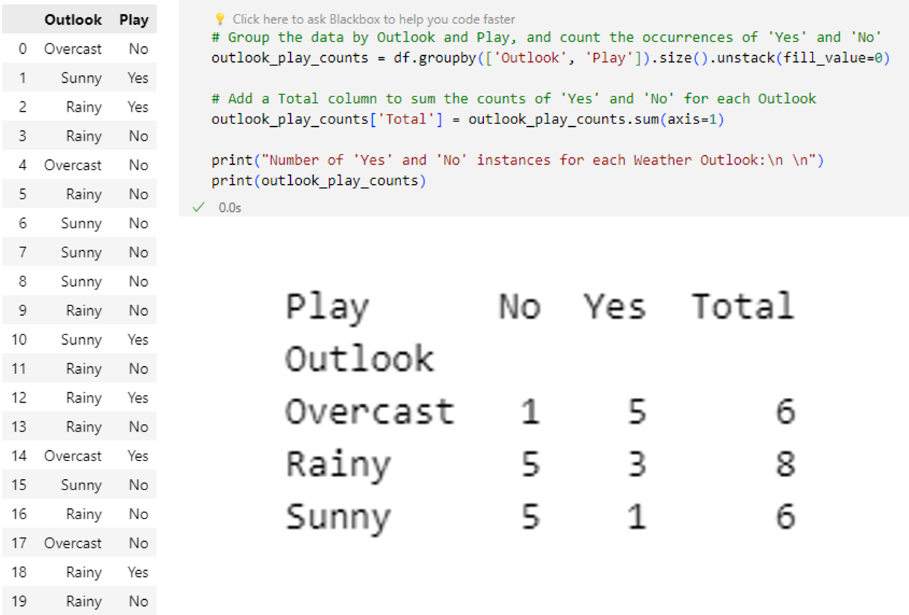
Example: Python implementationA Python implementation of this example with little bit changed outlooks:
        import pandas as pd
        import random

        # Define the possible values for Outlook and Play
        outlook_values = ['Sunny', 'Rainy', 'Overcast']
        play_values = ['Yes', 'No']

        # Generate 20 random data points
        data = {
            'Outlook': [random.choice(outlook_values) for _ in range(20)],
            'Play': [random.choice(play_values) for _ in range(20)]
        }
        df = pd.DataFrame(data)

        # Calculate the total number of instances
        total_instances = len(df)

        # Calculate the number of instances where the outlook is sunny
        sunny_instances = len(df[df['Outlook'] == 'Sunny'])

        # Calculate the number of instances where the outlook is sunny and the player plays
        sunny_play_instances = len(df[(df['Outlook'] == 'Sunny') & (df['Play'] == 'Yes')])

        # Calculate the prior probability of playing the game
        prior_probability_play = df['Play'].value_counts(normalize=True)['Yes']

        # Calculate the probability of playing the game given that the outlook is sunny using Bayes' theorem
        probability_play_given_sunny = (sunny_play_instances / sunny_instances) * prior_probability_play

        print("Probability of playing the game on a Sunny day using Bayes' theorem:", probability_play_given_sunny)
Probability of playing the game on a Sunny day using Bayes' theorem: 0.09999999999999999

Examples-2: Iris data
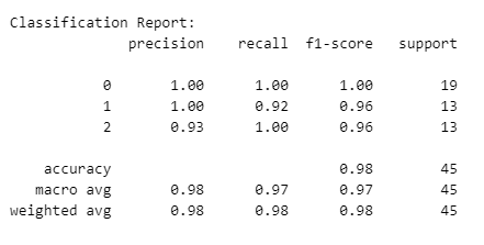
In this example. we consider the 'Iris' dataset. This example demonstrates the process of training and evaluating a Gaussian Naive Bayes classifier on the Iris dataset using scikit-learn. It shows how to load the data, split it into training and testing sets, train the classifier, make predictions, and evaluate the classifier's performance using accuracy, classification report, and Confusion matrix details.
        from sklearn.datasets import load_iris
        from sklearn.model_selection import train_test_split
        from sklearn.naive_bayes import GaussianNB
        from sklearn.metrics import classification_report, confusion_matrix

        # Load the Iris dataset
        iris = load_iris()
        X = iris.data
        y = iris.target

        # Split the dataset into training and testing sets
        X_train, X_test, y_train, y_test = train_test_split(X, y, test_size=0.3, random_state=42)

        # Initialize the Gaussian Naive Bayes classifier
        gnb = GaussianNB()

        # Train the classifier
        gnb.fit(X_train, y_train)

        # Make predictions on the testing set
        y_pred = gnb.predict(X_test)
        # Calculate the accuracy of the classifier
        accuracy = gnb.score(X_test, y_test)
        print("Accuracy:", accuracy)
Accuracy: 0.9777777777777777
        # Print classification report and confusion matrix
        print("\nClassification Report:")
        print(classification_report(y_test, y_pred))

Confusion matrix:
        print("\nConfusion Matrix:")
        print(confusion_matrix(y_test, y_pred))

The classification report provides a concise summary of the performance of a classifier. In this report, precision measures the accuracy of positive predictions, recall assesses the proportion of actual positives correctly identified, and the F1-score balances precision and recall. For the given classes (0, 1, 2), the classifier achieves high precision, indicating accurate positive predictions. Similarly, recall scores show effective identification of actual positives, though class 1 has slightly lower recall. The F1-score reflects a good balance between precision and recall for each class, indicating overall strong performance. The support values represent the number of instances for each class in the testing set. The reported accuracy of 98% highlights the overall correctness of the classifier across all classes, with both macro and weighted averages reinforcing balanced performance.
Example-3
In this example, we use dataset 'User_Data.csv' for training, or testing algorithms like Naive Bayes for classification tasks. In this case, it provides a starting point for implementing a Naive Bayes algorithm using Python. Data is available in my Github repo- Step-1: Generate a random dataset:
            import pandas as pd
            import numpy as np
            import random
            import matplotlib.pyplot as plt

            df_user =  pd.read_csv('User_Data.csv')

            # Display the DataFrame
            print(df_user.head())

            # Display the DataFrame
            print(df_user.head())
                # Importing the dataset
                X = df_user.iloc[:, [2, 3]].values
                y = df_user.iloc[:, 4].values

                # Splitting the dataset into the Training set and Test set
                from sklearn.model_selection import train_test_split
                X_train, X_test, y_train, y_test = train_test_split(X, y, test_size = 0.25, random_state = 0)
                # Feature Scaling
                from sklearn.preprocessing import StandardScaler
                sc = StandardScaler()
                X_train = sc.fit_transform(X_train)
                X_test = sc.transform(X_test)
                # Fitting Naive Bayes to the Training set
                from sklearn.naive_bayes import GaussianNB
                classifier = GaussianNB()
                classifier.fit(X_train, y_train)
                # Predicting the Test set results
                y_pred = classifier.predict(X_test)
                # Making the Confusion Matrix
                from sklearn.metrics import confusion_matrix
                cm = confusion_matrix(y_test, y_pred)
            import numpy as np
            import matplotlib.pyplot as plt
            from matplotlib.colors import ListedColormap

            # Create a figure with two subplots
            fig, axes = plt.subplots(1, 2, figsize=(12, 5))

            # Plot for training set
            plt.sca(axes[0])  # Select the first subplot
            x_set, y_set = X_train, y_train
            X1, X2 = np.meshgrid(np.arange(start=x_set[:, 0].min() - 1, stop=x_set[:, 0].max() + 1, step=0.01),
                                 np.arange(start=x_set[:, 1].min() - 1, stop=x_set[:, 1].max() + 1, step=0.01))
            plt.contourf(X1, X2, classifier.predict(np.array([X1.ravel(), X2.ravel()]).T).reshape(X1.shape),
                         alpha=0.75, cmap=ListedColormap(('lightblue', 'lightgreen')))
            plt.xlim(X1.min(), X1.max())
            plt.ylim(X2.min(), X2.max())
            for i, j in enumerate(np.unique(y_set)):
                plt.scatter(x_set[y_set == j, 0], x_set[y_set == j, 1],
                            c=ListedColormap(('blue', 'green'))(i), label=j)
            plt.title('Naive Bayes (Training set)')
            plt.xlabel('Age')
            plt.ylabel('Estimated Salary')
            plt.legend()

            # Plot for test set
            plt.sca(axes[1])  # Select the second subplot
            x_set, y_set = X_test, y_test
            X1, X2 = np.meshgrid(np.arange(start=x_set[:, 0].min() - 1, stop=x_set[:, 0].max() + 1, step=0.01),
                                 np.arange(start=x_set[:, 1].min() - 1, stop=x_set[:, 1].max() + 1, step=0.01))
            plt.contourf(X1, X2, classifier.predict(np.array([X1.ravel(), X2.ravel()]).T).reshape(X1.shape),
                         alpha=0.75, cmap=ListedColormap(('lightblue', 'lightgreen')))
            plt.xlim(X1.min(), X1.max())
            plt.ylim(X2.min(), X2.max())
            for i, j in enumerate(np.unique(y_set)):
                plt.scatter(x_set[y_set == j, 0], x_set[y_set == j, 1],
                            c=ListedColormap(('blue', 'green'))(i), label=j)
            plt.title('Naive Bayes (Test set)')
            plt.xlabel('Age')
            plt.ylabel('Estimated Salary')
            plt.legend()

            # Adjust layout and display the plots
            plt.tight_layout()
            plt.show()

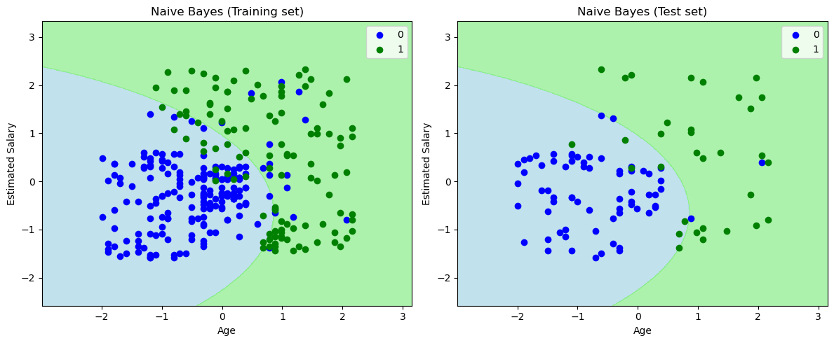
The final output above depicts the classifier's performance on the test set data. The classifier has effectively created a Gaussian curve to separate the "purchased" and "not purchased" variables, demonstrating its ability to classify the data. Despite some erroneous predictions, which are quantified in the confusion matrix, overall, the classifier demonstrates strong performance and can be considered a reliable predictor.
References
- My github Repositories on Remote sensing Machine learning
- Understanding Naive Bayes Classifier: Simplilearn.
- Naïve Bayes Classifier Algorithm, JAVAPoint.com
- Book on Statistics: The Elements of Statistical Learning
Some other interesting things to know:
- Visit my website on For Data, Big Data, Data-modeling, Datawarehouse, SQL, cloud-compute.
- Visit my website on Data engineering

