Sea Surface Temperature

Content
Home

Physical Quantity of Interest: Sea Surface Temperature

Before discussing satellite instruments or algorithms, it is important to define the geophysical quantity of interest. Sea Surface Temperature (SST) refers to the temperature of the ocean at or near the interface between the ocean and the atmosphere. However, this seemingly simple definition hides important physical distinctions.

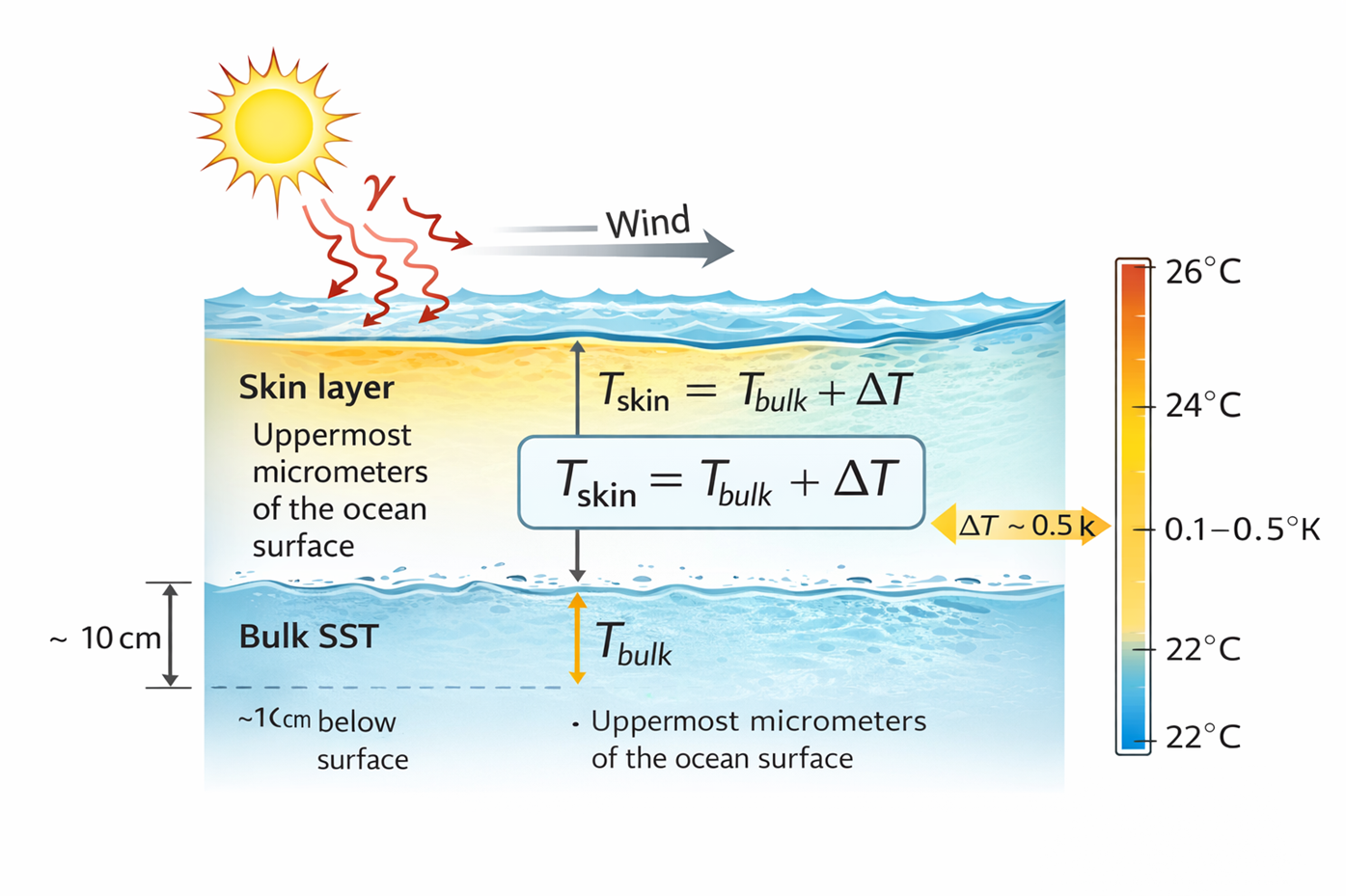
Satellite infrared radiometers are sensitive to radiation emitted from the uppermost micrometres of the ocean surface, commonly referred to as the skin layer. The temperature inferred from thermal infrared measurements is therefore the skin SST, denoted $T_{\text{skin}}$. In contrast, in-situ measurements from buoys or ships typically represent the bulk SST, measured at depths of order centimetres to meters, denoted $T_{\text{bulk}}$.

The relationship between these quantities can be expressed schematically as:

$$T_{\text{skin}} = T_{\text{bulk}} + \Delta T$$

where $\Delta T$ represents the skin–bulk temperature difference, influenced by factors such as wind speed, solar heating, and turbulent mixing. This difference is typically small (on the order of a few tenths of a kelvin) but is not negligible for climate applications.

Satellites cannot measure SST directly. Instead, they observe thermal infrared radiance emitted by the ocean–atmosphere system. This radiance depends not only on surface temperature but also on atmospheric absorption and emission, surface emissivity, and viewing geometry. As a result, SST must be estimated indirectly by solving an inverse problem that links observed radiance to surface temperature through physical models.

Despite these limitations, SST is one of the most widely used satellite-derived geophysical variables. It plays a central role in:

numerical weather prediction, where SST influences air–sea heat and moisture fluxes,
ocean circulation and air–sea interaction studies,
detection and analysis of climate variability and long-term trends,
marine ecosystem and biogeochemical applications.

Because SST sits at the intersection of physics, observation, and modelling, it provides an ideal framework for illustrating the complexity and logic of satellite data processing chains.

Governing Thermodynamic Description of Sea Surface Temperature

To understand Sea Surface Temperature (SST) mathematically, we must view it as the thermodynamic result of the energy balance at the interface between the ocean and the atmosphere. In physical oceanography, SST is not a single value but a vertical profile. We differentiate between the Skin Temperature $\text{SST}_{\text{skin}}$ and the Bulk Temperature $\text{SST}_{\text{bulk}}$.

Temperature as a Prognostic Variable

The ocean temperature field is a continuous function of space and time: $$T = T(x, y, z, t)$$ where,

$x, y$ are horizontal coordinates,
$z$ is vertical depth (positive downward),
$t$ is time.

Temperature evolution in the ocean is governed by energy conservation.

Heat Conservation Equation (First Law of Thermodynamics)

The local rate of change of temperature is governed by the heat equation: $$ \rho c_p \frac{\partial T}{\partial t} = - \nabla \cdot \mathbf{F}_{\text{heat}} + Q $$ where:

$\rho$ is seawater density,
$c_p$ is specific heat capacity,
$\mathbf{F}_{\text{heat}}$ is the heat flux vector,
$Q$ represents internal heat sources (usually negligible near the surface).

Decomposition of Heat Flux

The heat flux consists of advective and diffusive components: $$ \mathbf{F}_{\text{heat}} = \rho c_p \mathbf{u} T - k \nabla T $$ where:

$\mathbf{u}$ is the fluid velocity,
$k$ is thermal conductivity (or turbulent diffusivity).

Substituting: $$ \frac{\partial T}{\partial t} + \mathbf{u} \cdot \nabla T = \nabla \cdot (\kappa \nabla T) $$ This is the advection–diffusion equation for temperature.

Near-Surface Vertical Structure

Near the ocean surface, vertical gradients dominate over horizontal gradients. We simplify: $$ \frac{\partial T}{\partial t} \approx \frac{\partial}{\partial z} \left( \kappa \frac{\partial T}{\partial z} \right) $$ This approximation is valid within the upper few centimeters, where molecular and turbulent diffusion dominate.

Boundary Condition at the Air–Sea Interface

At the surface $(z = 0)$, the vertical heat flux is set by the net air–sea heat exchange: $$ - k \frac{\partial T}{\partial z}\Big|_{z=0} = Q_{\text{net}} $$ where: $$Q_{\text{net}}= Q_{\text{sw}} - Q_{\text{lw}} - Q_{\text{sens}} - Q_{\text{lat}}$$ This boundary condition couples ocean thermodynamics to the atmosphere.

Formation of the Skin Layer

In the uppermost micrometers, turbulent mixing vanishes and molecular diffusion dominates. Under quasi-steady conditions: $$ \frac{\partial}{\partial z} \left( k \frac{\partial T}{\partial z} \right)= 0 $$ which integrates to a linear gradient: $$\frac{\partial T}{\partial z} = -\frac{Q_{\text{net}}}{k}$$

Skin–Bulk Temperature Difference

Integrating over the skin layer thickness $\delta$: $$T_{\text{skin}} - T_{\text{bulk}} = - \int_0^{\delta} \frac{Q_{\text{net}}}{k}, dz$$ which yields: $$ \boxed{ \Delta T = T_{\text{skin}} - T_{\text{bulk}} \approx - \frac{Q_{\text{net}}}{\rho c_p u_*} } $$ where $u_*$ is the friction velocity, representing turbulent exchange.

This equation explains why:

low wind → strong skin cooling,
high wind → reduced skin–bulk difference.

Definition of Satellite-Relevant SST

Thermal infrared satellites sense radiation emitted from the skin layer, therefore: $$T_{\text{sat}} \equiv T_{\text{skin}} = T(z \rightarrow 0^+)$$ This is a boundary value, not a vertically averaged temperature.

Radiative Expression of Skin Temperature

The skin temperature enters the radiation field via Planck’s law: $$ B(\lambda, T_{\text{skin}}) = \frac{2hc^2}{\lambda^5} \frac{1}{\exp\left(\frac{hc}{\lambda k T_{\text{skin}}}\right)-1} $$ The emitted ocean radiance is: $$L_{\text{surf}}(\lambda) = \varepsilon(\lambda) B(\lambda, T_{\text{skin}})$$

Atmosphere–Ocean Coupled Observation Equation

Including atmospheric effects: $$ L_{\text{TOA}}(\lambda) = \tau(\lambda) \varepsilon(\lambda) B(\lambda, T_{\text{skin}}) + L_{\text{atm}}^{\uparrow}(\lambda) $$ This is the forward physical model linking thermodynamics to satellite observations.

Observed Quantity and Inversion Target

The satellite measures channel-integrated radiance: $$L_c = \int L_{\text{TOA}}(\lambda) R_c(\lambda) d\lambda$$ The retrieval problem is: $$ \boxed{ \text{Given } L_c \Rightarrow \text{Estimate } T_{\text{skin}} } $$ This is an inverse problem, constrained by thermodynamics, radiative transfer, and statistics.

Conceptual Closure

Starting from the heat equation, we have shown that:

SST is governed by energy conservation
The skin temperature emerges from surface boundary conditions.
Satellites sense a thermodynamic boundary layer.
SST retrieval is fundamentally a physics-based inversion.

This framework ensures that SST is understood not as a “product”, but as the solution of a coupled thermodynamic–radiative system.

Derivation of the Split-Window SST Algorithm

The split-window sea surface temperature (SST) algorithm is one of the most widely used techniques for deriving SST from thermal infrared satellite observations. It exploits measurements from two closely spaced infrared channels, typically near 11 µm and 12 µm, which have similar sensitivity to surface temperature but different sensitivity to atmospheric absorption, primarily by water vapour.

The key idea of the split-window approach is that the difference between the brightness temperatures measured in these two channels provides a proxy for the atmospheric contribution to the observed radiance. By combining the channel brightness temperatures in a linear form, the algorithm largely cancels atmospheric effects while preserving the surface temperature signal.

Although often introduced as an empirical formula, the split-window algorithm can be derived rigorously by linearising the radiative transfer equation around a reference temperature. This reveals that the algorithm is a first-order approximation to the inverse problem of retrieving surface temperature from top-of-atmosphere radiance, with coefficients that reflect atmospheric transmittance, emissivity, and instrument characteristics.

Error Propagation and Climate Stability Implications

Forward Radiative Transfer Model (Starting Point):

From the thermodynamic discussion, the top-of-atmosphere (TOA) radiance in an infrared channel (i) is:

$$L_i = \tau_i \varepsilon_i B(T_{\text{skin}}) + L_{i}^{\uparrow}$$ where:

$B(T)$ is the Planck function (channel-integrated
$T_{\text{skin}}$ is the sea surface skin temperature,
$\tau_i$ is atmospheric transmittance,
$\varepsilon_i$ is surface emissivity,
$L_{i}^{\uparrow}$ is upwelling atmospheric emission.

The satellite does not observe $T_{\text{skin}}$, but the radiance $L_i$. To simplify notation, define: $A_i = \tau_i \varepsilon_i$, so $$ L_i = A_i B(T_{\rm skin}) + L_{i}^{\uparrow} $$

Brightness Temperature Representation:

Brightness temperature $T_{b,i}$ is defined implicitly by: $$L_i = B_i(T_{b,i})$$ where $B_i(\cdot)$ is the Planck function integrated over the channel response. So, $$ B(T_{b,i}) = A_i B(T_{\rm skin}) + L_{i}^{\uparrow} $$ This equation is exact.

Linearize Around a Reference Temperature $T_0$:

Let both temperatures be clos to a reference $T_0$. Now definin the two temperatures as:

$$T_{\rm skin} = T_0 +\delta T_s$$ $$T_{b,i} = T_0 +\delta T_{b,i}$$

Now expand Planck’s function using a first-order Taylor expansion:

$$ B(T) \approx B(T_0) + B' (T_0) (T - T_0). $$

Now applying this to both sides. The left hand side:

$$B(T_{b,i}) \approx B(T_0) + B'(T_0) \delta T_{b,i}.$$

and the right hand side:

$$A_i [B(T_0) + B'[T_0]\delta T_s] + L_{i}^{\uparrow}$$

Now, equating both sides:

$$ B(T_0) + B'(T_0) \delta T_{b,i} = A_i B(T_0) + A_i B'(T_0) \delta T_s + L_{i}^{\uparrow} $$ Now rearranged: $$ B'(T_0) \delta T_{b,i} A_i B'(T_0) \delta T_s + (A_i -1) B(T_0) + L_{i}^{\uparrow} $$ Now divide by $B'(T_0)$, $$ \delta T_{b,i} = A_i \delta T_s + \frac{(A_i -1) B(T_0)}{B(T_0)} + \frac{L_{i}^{\uparrow}}{B'(T_0)}. $$

Now recalling $\delta T_{b,i} = T_{b,i} - T_0$ and $\delta T_{s} = T_{\rm skin} - T_0$. Therefore, above equation can be rearranged to:

$$ T_{b,i} = T_0 + A_i (T_{\rm skin} - T_0) +C_i $$

where,

$$ C_i = \frac{(A_i -1) B(T_0)}{B'(T_0)} + \frac{L_{i}^{\uparrow}}{B'(T_0)} $$ Therefore, we can rearranging again: $$T_{b,i} = A_i T_{\rm skin} + \beta_i$$

where

$$\beta_i = T_0 (1- A_i) +C_i .$$

Physical Interpretation:

This shows that brightness temperature is approximately:

$$T_{b,i} = A_i T_{\rm skin} + \beta_i$$

where:

$A_i < 1$ because atmoshphere absorbs
$\beta_i$ contains atmospheric emission and constant offsets

This is the correct linearized relationship.

Why Split-Window Works? For two channels, i.e.

channel 1: $ \lambda_1 \approx 11 ,\mu\text{m} $
channel 2: $ \lambda_2 \approx 12 ,\mu\text{m} $

$$T_{b,1} = A_1 T_s + \beta_1 $$ $$T_{b,2} = A_2 T_s + \beta_2$$ subtract: $$T_{b,1}- T_{b,2} = (A_1 - A_2) T_s + (\beta_1 - \beta_2)$$

Since atmospheric absorption differs slightly between channels, this difference isolates atmospheric effects, allowing us to construct a linear estimator for $T_s$. We can solve these two equations for $T_s$ as:

$$T_s = \frac{T_{b,1} - \beta_1}{A_1} = \frac{T_{b,2} - \beta_2}{A_2}.$$

But in reality, $\beta_i$ and $A_i$ depend on atmospheric state and are not known perfectly. So instead of solving exactly, we build a first-order linear estimator that compensates for atmospheric effects using the brightness temperature difference. That estimator is:

$$T_s = a_0 +a_1 T_{b,1} + a_2 (T_{b,1} - T_{b,2}).$$

This is the split-window SST equation. Where:

$T_{b,1}$ contains mostly surface signal
$T_{b,1} - T_{b,2}$ isolates atmospheric abosrption
A linear combination cancels first-order atmospheric effects.

These coefficients $a_0$, $a_1$, $a_2$ are determined from radiative transfer simulations, regression against in-situ SST, or analytical approximation from the linearized forward model

Many operational algorithms use:

$$T_s = T_{b,1} + c_1 (T_{b,1} - T_{b,2}) +c_0$$ and sometimes additional terms are added, for example: $$T_s = T_{b,1} + c_1 (T_{b,1} - T_{b,2}) + c_2 (T_{b,1} - T_{b,2})^2 + c_0$$ That is the split-window SST equation, which can be re-written in linear format as: $$Y_s = a+0 +\gamma_1 T_{b,1} + \gamma_2 T_{b,2},$$

where $\gamma_1 = a_1 +a_2$ and $\gamma_2 = -a_2$

Error Covariance and Uncertainty Propagation:

Brightness Temperature Error Model Let the measured brightness temperature be:

$$T_{b,i}^{\rm obs} = T_{b,i}^{\rm true} + \varepsilon_i$$ where: $$\varepsilon_i = \varepsilon_{\text{noise},i}+ \varepsilon_{\text{cal},i} + \varepsilon_{\text{model},i}.$$

Each $\varepsilon_i$ is a random variable. Define vector:

$$ \varepsilon = \begin{bmatrix} \epsilon_1 \\ \epsilon_2 \end{bmatrix} $$

Error Covariance Matrix of Brightness Temperatures: Define:

$$ \mathbf{S}_b = \mathrm{Cov}\left(\boldsymbol{\epsilon}\right) = \begin{bmatrix} \sigma_1^2 & \sigma_{12} \\ \sigma_{12} & \sigma_2^2 \end{bmatrix} $$ where

$\sigma_1^2 = \text{Var}(\epsilon_1)$
$\sigma_2^2 = \text{Var}(\epsilon_2)$
$\sigma_{12} = \text{Cov}(\varepsilon_1, \varepsilon_2)$

This covariance term is critical.

Linear Uncertainty Propagation: Because SST is linear in brightness temperatures:

$$T_s =\mathbf{g}^T \mathbf{T}_b + a_0$$ where: $$ \mathbf{g} = \begin{bmatrix} \gamma_1 \\ \gamma_2 \end{bmatrix} $$

Then the variance of SST is:

$$\boxed{\sigma_{T_s}^2 = \mathbf{g}^T \mathbf{S}_b \mathbf{g}}$$

This is the matrix form of the law of propagation of uncertainty. This can be expanded explicitly:

$$\sigma_{T_s}^2 = \gamma_1^2 \sigma_1^2 + \gamma_2^2 \sigma_2^2 + 2 \gamma_1 \gamma_2 \sigma_{12}$$ This is the full propagation equation.

Why the Covariance Term Matters:

If errors are independent: $$ \sigma_{12} = 0 $$ But in reality:

Calibration drift: If both channels share calibration reference:

$$ \epsilon_{\text{cal},1} \approx \epsilon_{\text{cal},2} $$ Then: $$ \sigma_{12} \approx \sigma_{\text{cal}}^2 $$ This introduces strong correlation. Ignoring covariance can:

underestimate SST uncertainty
misrepresent long-term stability

Brightness temperature errors consist of: $$\epsilon_{b,i} = \epsilon_{\text{noise},i} + \epsilon_{\text{cal},i} + \epsilon_{\text{model},i}$$

Decomposition of Error Contributions:

Total brightness error: $$ \mathbf{S}_b = \mathbf{S}_{\text{noise}} + \mathbf{S}_{\text{cal}}+\mathbf{S}_{\text{model}} $$

Instrument noise: Usually independent: $$ \mathbf{S}_{\text{noise}} = \begin{bmatrix} \sigma_{n1}^2 & 0 \\ 0 & \sigma_{n2}^2 \end{bmatrix} $$
Calibration error: Often fully correlated: $$ \mathbf{S}_{\text{cal}} = \sigma_{\text{cal}}^2 \begin{bmatrix} 1 & 1 \\ 1 & 1 \end{bmatrix} $$
Forward model error: Partially correlated: $$ 0 < \rho < 1 $$ $$ \mathbf{S}_{\text{model}} = \begin{bmatrix} \sigma_{m1}^2 & \rho \sigma_{m1} \sigma_{m2} \\ \rho \sigma_{m1} \sigma_{m2} & \sigma_{m2}^2 \end{bmatrix} $$

Impact on SST Stability:

Let SST bias drift over time be: $b(t)$. The Observed SST: $$ \hat{T}_s(t) = T_s(t) + b(t) $$ climate trend: $$\frac{d\hat{T}_s}{dt} = \frac{dT_s}{dt} + \frac{db}{dt}$$ If calibration drift induces: $$\frac{db}{dt} \sim 0.02 \text{ K decade}^{-1}$$ and climate signal is: $$\frac{dT_s}{dt} \sim 0.1 \text{ K decade}^{-1} $$ then 20% of the trend may be instrument artifact.

Reference

Go to Content