
Understanding Satellite Systems and the Complexity of data Processing Chains
Introduction
Modern satellite missions observe the Earth continuously, producing vast amounts of data that support weather forecasting, climate monitoring, and environmental research. However, satellite data are not directly usable when they are first received on the ground. Instead, they pass through a multi-stage data processing chain, where raw instrument measurements are transformed into geophysical products such as temperature, humidity, trace gas concentrations, or ocean surface properties. This transformation involves complex systems and coordinated efforts among multiple technical and scientific teams. This transformation relies on sophisticated data processing chains, which are both technically complex and scientifically essential.
What a Satellite Actually Measures
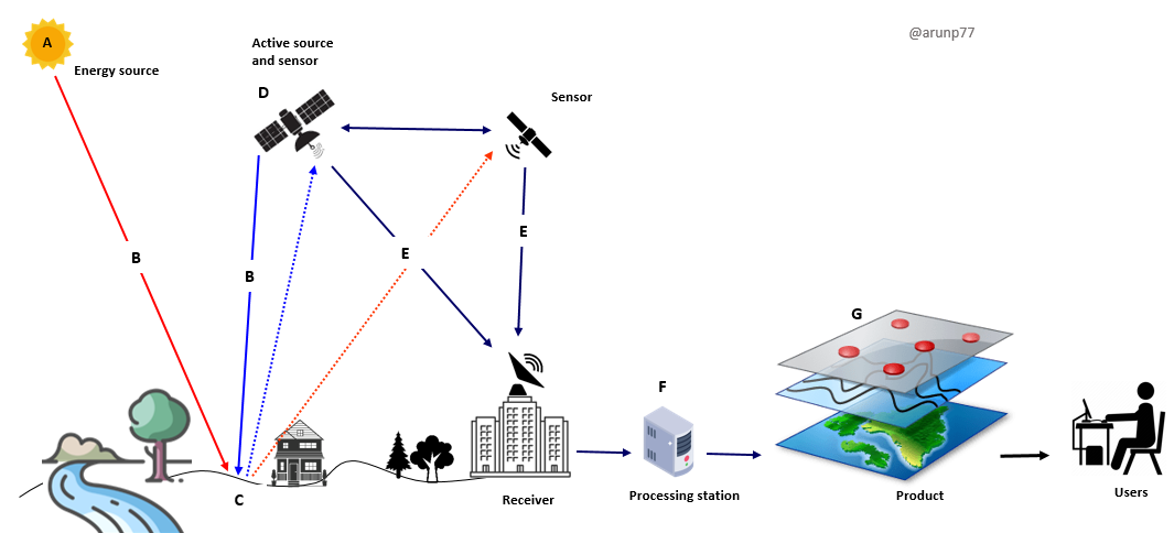
Satellite instruments do not measure geophysical variables directly. Instead, they measure electromagnetic radiation reaching the sensor at the top of the atmosphere. Depending on the instrument, this radiation may be reflected sunlight (visible and near-infrared) or thermal emission from the Earth–atmosphere system (infrared and microwave).
The fundamental measured quantity is usually spectral radiance, integrated over the spectral response of a sensor channel. In simplified form, the sensor output can be written as
$$C = f(L) + \epsilon $$ where- \(C\) is the recorded digital count (or digital number),
- \(L\) is the true radiance reaching the instrument,
- \(f(.)\) represents the sensor response (gain, offset, non-linearity),
- \(\epsilon\) represents measurement noise and unmodelled effects.
These raw counts are the starting point of the processing chain.
Journey (High-Level Flow)
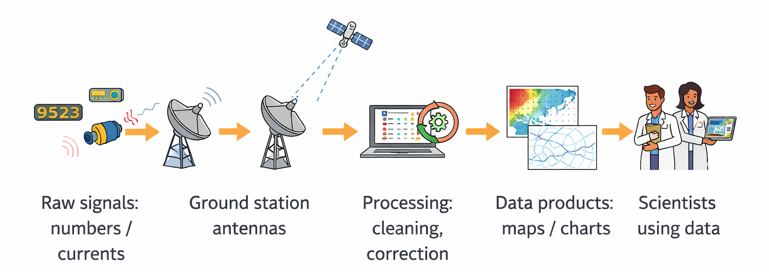
Mission Goals → Satellite Design → Launch → Data Reception → Data Processing → Research
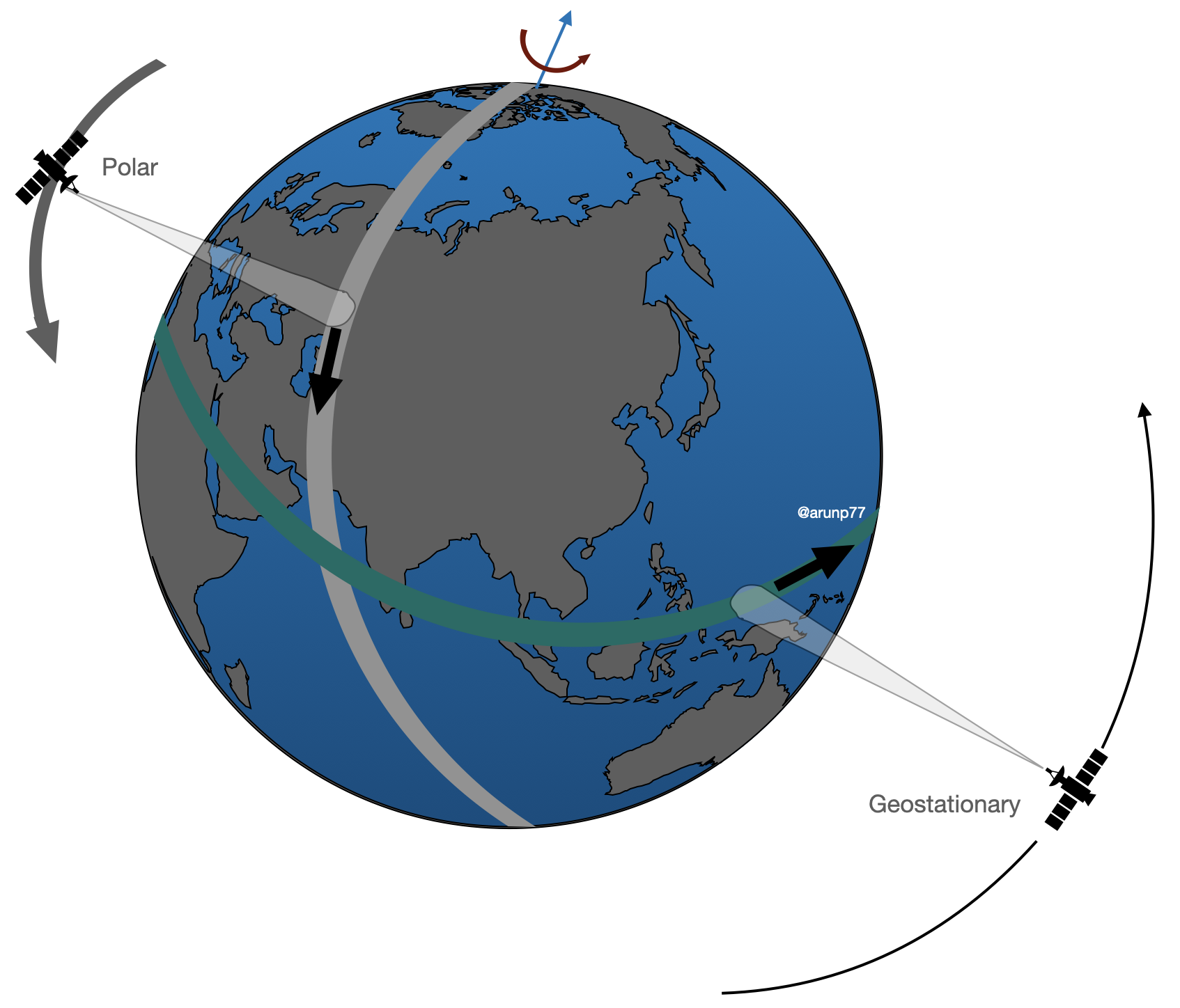
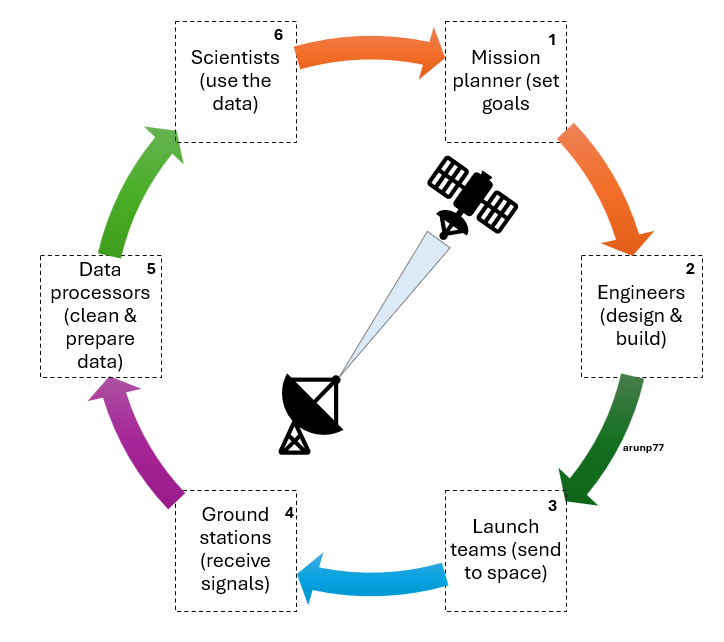
Image credit: © Arun Kumar Pandey
The Backbone: Satellite Systems
Modern Earth observation (EO) satellites, such as the METOP-SG or Sentinel series from the Copernicus program, are equipped with an array of instruments. These include radiometers, spectrometers, and radar sensors that collect data across various spectral ranges and spatial resolutions. Instruments like IASI (Infrared Atmospheric Sounding Interferometer) and SAR (Synthetic Aperture Radar) capture voluminous raw data with high temporal and spatial fidelity.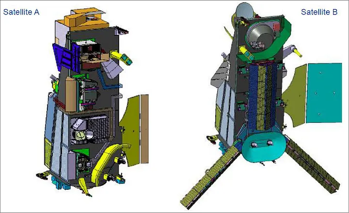
However, these instruments merely initiate the data chain. What follows is a sophisticated multi-tiered processing pipeline that transforms these bits and bytes into meaningful insights.
The Data Processing Chain: From Bits to Insight
Onboard Processing and Transmission
The process starts with satellite instruments measuring Earth system parameters. Minimal preprocessing occurs onboard (such as data compression and time tagging) before the telemetry is transmitted to ground stations.
To manage complexity and responsibilities, satellite data are conventionally grouped into processing levels. While exact definitions vary between agencies, the general structure is well established.
- Level 0: Raw Data Reception Once transmitted to ground stations, the satellite data are received in their rawest form, often including telemetry,
ancillary data, and mission-specific housekeeping information.
At this stage, the data are not calibrated and have little direct scientific meaning. Digitisation already imposes a fundamental limit on precision. For example, an \(N\)-bit analogue-to-digital converter introduces a quantisation uncertainty of approximately $$\sigma_{\text{digit}}= \frac{1}{\sqrt{12}} \Delta$$ where \(\Delta\) is the quantisation step.
-
Level 1: Calibration and Geolocation
The next step involves converting the raw measurements into physical units (e.g., radiance or reflectance), correcting for instrument-specific biases and
geometric distortions. This calibration and geolocation process is crucial to ensure that the data are both accurate and traceable to physical ground locations.
A simplified calibration equation for one channel can be written as:
$$L = a+0+a_1 C +a_2 C^2$$ where,- \(L\) is the calibrated radiance,
- \(C\) is the measured count,
- \(a_0\), (a_1\) and (a_2\) are calibration parameters (offset, gain, non-linearity).
Calibration parameters are derived from pre-launch characterisation and in-flight calibration sources (e.g. blackbodies or solar diffusers). Over time, sensor degradation and changing thermal conditions introduce drift, making long-term stability a major challenge.
Uncertainty in L1 radiances arises from:
- detector noise,
- calibration parameter uncertainty,
- digitisation,
- imperfect knowledge of the sensor response.
-
Level 2: Derived Geophysical Variables
At this stage, the calibrated measurements are converted into geophysical parameters such as surface temperature, cloud cover, ocean salinity, or greenhouse gas
concentrations. This step often involves radiative transfer models and retrieval algorithms that integrate information from multiple sensors and external databases.
Level 2 products estimate geophysical quantities such as temperature, humidity, or trace gas concentration from L1 radiances. This step is an inverse problem, often written as: $$z=g(y,b) + \delta$$ where,
- \(z\) is the retrieved geophysical state,
- \(y\) is the vector of observed radiances,
- \(b\) represents auxiliary data and model parameters,
- \(g\) is the retrieval algorithm,
- \(\delta\) epresents residual modelling error.
Subsequent levels involve spatial and temporal aggregation, gridding, and fusion with data from other sources (e.g., in-situ or model data). These higher-level products are designed for direct use in scientific analyses, weather forecasting models, and policy-making dashboards.
-
Level 3 (L3): Gridded Products:
Level 3 products reorganise L2 data onto a fixed spatial and/or temporal grid. This often involves averaging: $$\bar{z} = \frac{\sum_{i=1}^N w_i z_i}{\sum_{i=1}^N w_i}$$ whee \(z_i\) are individual L2 observations and \(w_i\) are weights based on quality or sampling.
While averaging reduces random noise, it does not necessarily reduce correlated errors. In addition, L3 products introduce sampling uncertainty, because irregular satellite observations are used to represent continuous geophysical fields.
-
Level 4 (L4): Gap-Filled and Model-Integrated Products:
Level 4 products combine satellite data with models and/or in situ observations to produce spatially and temporally complete fields. These products are highly useful but are no longer purely observation-based. Their uncertainty reflects a mixture of measurement error, model assumptions, and interpolation choices.
Propagation of Uncertainty Through the Chain
A central concept in satellite data processing is that uncertainty propagates through each processing step. For a measurement function.
$$y = f(x_1,x_2,...,x_n)$$the standard uncertainty in \(y\) can be approximated using the Law of Propagation of Uncertainty:
$$\sigma_y^2 = \sum_{ij} \frac{\partial f}{\partial_i}\frac{\partial f}{\partial_j}$$This expression highlights why error correlations matter. Ignoring covariance terms can lead to under- or overestimation of uncertainty, especially in gridded and climate-scale products.
Challenges in the Chain
Maintaining the fidelity and integrity of data throughout this processing pipeline is a non-trivial engineering and scientific challenge. Issues such as file size inconsistencies, synchronization errors, and processor-specific variations (e.g., between different ground segments or missions) can affect data quality. These anomalies must be continuously monitored, understood, and resolved.
Additionally, with growing demands for near real-time (NRT) products, latency and computational throughput have become critical parameters. Data processing systems must therefore be scalable, fault-tolerant, and optimized for high-performance computing environments.
Collaboration Across Specialized Teams
The successful generation and delivery of satellite products depend on close collaboration between diverse teams, each with unique responsibilities:
- Instrument and Engineering Teams: These teams understand the behavior of onboard instruments and provide support for calibration algorithms, noise handling, and anomaly detection. They are also responsible for instrument-specific configurations in the processor chains.
- Data Processing and Software Engineering Teams: These teams design and maintain the ground processing systems and algorithms. They handle tasks like performance tuning, software validation, and ensuring consistent file formats and metadata structures.
- Validation and Verification Teams (IV&V): Independent teams evaluate whether processing chains meet scientific and operational requirements. They analyze outputs for accuracy, quality, and compliance with mission specifications.
- Data Quality Control and Monitoring Teams: These groups continuously monitor the outputs, investigate anomalies, and flag inconsistencies. For instance, they might identify unexpected variations in file sizes or processing delays and coordinate with upstream teams to resolve them.
- Archiving and Distribution Teams Once products are validated, they are archived and distributed through systems like EUMETSAT’s EUMETCast or UMARF (Unified Meteorological Archive and Retrieval Facility), making them accessible to end users.
Importance of Coordination and Robust Infrastructure
The seamless functioning of this ecosystem depends on robust documentation, regular coordination meetings, and shared monitoring tools. For example, dashboards may display the status of each processing node, enabling quick detection of bottlenecks. Reporting systems highlight gaps (e.g., files sent to EDL but not archived), which teams investigate collaboratively.
In large operations like EPS-SG, issues such as mismatched file counts, varying file sizes, or missing data often involve cross-functional inputs. Resolving these requires a systems-thinking approach and transparency across teams.
Why This Matters?
Understanding and investing in satellite data processing chains is not merely a technical requirement; it is foundational to the credibility and applicability of satellite-derived information. These chains are essential for:
- Climate Research: Long-term, consistent data records support climate trend analysis and predictive modeling.
- Disaster Management: Rapid data delivery enables timely responses to natural hazards like hurricanes, wildfires, and floods.
- Agricultural and Water Resources Monitoring: High-resolution datasets inform irrigation planning, crop yield estimation, and drought assessment.
- Policy and Governance: Trustworthy data support evidence-based policy decisions at national and international levels.
Conclusion
The sophistication of satellite systems and their data processing chains reflects the complexity of the Earth systems they monitor. Scientists and engineers alike must collaborate to ensure that every byte of data collected in space contributes meaningfully to our understanding and stewardship of the planet. As our need for timely, accurate Earth observation grows, so too must our investment in the integrity and performance of these critical processing infrastructures.
Reference
- Fundamentals of Remote sensing
- Relevance of Electromagnetic waves in the context of earth observation
- Concept of the orbits for a satellite (non scientific discussion)
- How various teams works in close collaboration for the ground data processing?
- How raw satellite data is processed to do a level where you do your scientifc research?
- In depth understandingof the satellite data (op-of-atmosphere reflectance)
- Resolution and calibration
- Understanding how OLCI data is processed
- Transforming Energy into Imagery: How Satellite Data Becomes Stunning Views of Earth