
Principal component analysis (PCA)
Introduction
Imagine you're working on a big data project, and the dataset contains numerous features. As you initiate your analysis, you may encounter situations where many features are correlated, leading to uncertainty about which features to choose for your analysis. Running a model, such as Regression or another, on the entire dataset may result in poor accuracy, leaving you in a challenging position.
In response, you might consider employing strategic methods to identify important variables. Techniques like Ridge, Lasso, and Elasticnet, known as regularization methods, can help prevent overfitting in machine learning models by adding penalty terms to the loss function. These methods primarily operate with the existing features. On the other hand, Principal Component Analysis (PCA) takes a different approach. It is a dimensionality reduction technique that transforms the original features into a new set of uncorrelated features called principal components. PCA proves beneficial when dealing with a large number of features, providing a way to reduce them while retaining most of the variability in the data.
In summary, while Ridge, Lasso, and Elastic Net focus on regularization, PCA focuses on reducing dimensionality, which can be beneficial in situations with a high number of features or multicollinearity. Statistical techniques such as factor analysis and PCA help to overcome such difficulties of choosing important features. (Look at following book for reference: Reference-4).
Defining PCA
Principal component analysis (PCA) is a statistical procedure that is commonly used to reduce the dimensionality of large data sets. It does this by transforming the data into a new coordinate system where the new variables are linear combinations of the original variables. The new variables are chosen so that they capture the most variance in the data.Why PCA is useful?
PCA is useful for several reasons:- Dimensionality reduction: PCA can be used to reduce the dimensionality of large data sets, which can make them easier to analyze and visualize.
- Data visualization: PCA can be used to visualize high-dimensional data in a way that is easy to understand.
- Linear Transformation: PCA performs a linear transformation of data, seeking directions of maximum variance.
- Feature extraction: PCA can be used to extract the most important features from a data set. This can be useful for tasks like classification and clustering by reducing noise and highlights underlying structure. Principal components are ranked by the variance they explain, allowing for effective feature selection.
- Data Compression: PCA can compress data while preserving most of the original information.
Applications of PCA
PCA has a wide range of applications in various fields, including:- Machine learning: PCA is a common preprocessing step in machine learning algorithms. It can be used to reduce the dimensionality of training data, which can improve the performance of the algorithm.
- Image analysis: PCA can be used to analyze and compress images. For example, it can be used to reduce the number of pixels in an image without losing much information.
- Finance: PCA can be used to analyze financial data, such as stock prices and returns. It can be used to identify patterns in the data and to make predictions about future prices.
- Chemistry: PCA can be used to analyze chemical data, such as spectra and molecular structures. It can be used to identify new compounds and to understand the relationships between different compounds.
Limitations of PCA
PCA is a powerful tool, but it also has some limitations:- PCA is based on the assumption that the data is Gaussian. This means that the data should be normally distributed. If the data is not normally distributed, PCA may not be able to accurately capture the most important features of the data.
- PCA is not scale-invariant. This means that the results of PCA can be sensitive to the scale of the variables. If the variables are measured on different scales, PCA may not be able to identify the most important features of the data.
Practical example
Let's consider a secanrio, you have a datasets of dimention \(\text{row} \times \text{columns} = \) \((n = 1000) \times (p = 40)\). These 40 columns represents possible features. But not all columns can be considered to be a feature. There are total row \(p \times (p-1)/2 =780\) numbers of scattered plots one can generate to see the possible relationships between the features. So it's almost impossible to find the relationships between the variables. In this case, the correlation of all these can actually gives you the clear image of the important features for your model.One possibility is to select a subset of the features which captures most of the variance. This can be done by looking at the explained variation ratio (EVR). After calculating the EVR, you can plot a cumulative sum of the explained variance. This plot, often referred to as the 'scree plot,' helps visualize how much variance in the data is retained as you include more principal components.
Next, you can set a threshold for the cumulative explained variance that you find acceptable. For example, you might decide to retain 95% of the variance. The corresponding number of principal components that cross this threshold gives you the optimal number of features to keep.
Once you determine the number of principal components to retain, you can use them to transform your original dataset into a reduced-dimensional space. This new dataset contains only the selected principal components, effectively reducing the number of features while retaining most of the information.
It's important to note that PCA assumes that the features are centered (have a mean of zero) and have similar scales. Therefore, it's a good practice to standardize or normalize the data before applying PCA.
In summary, PCA is a powerful tool for dimensionality reduction, particularly when dealing with a large number of features. It helps in identifying and retaining the most important information, making your data more manageable for further analysis or model training
What Are Principal Components?
Principal components are the orthogonal (uncorrelated) linear combinations of the original features in a dataset. These components are ordered by the amount of variance they explain in the data.The principal components are obtained through linear combination of the original variables. Let's say you have a dataset with variables \(X_1, X_2, ..., X_p\), and you can find the first principal component, denoted as \(PC_1\). The formula for \(PC_1\) is:
$$PC_1 = a_1 X_1 +a_2 X_2 + ... +a_p X_p$$here \(a_1, a_2, ..., a_p\) are the weights or coefficients assigned to each original variable, and they are choosen in such as a way that \(PC_1\) captures the maximum variance in the data. The weights are determined by solving an optimization problem, specified by finidng the eigne vectors of the covariance matrix of the original variables. The subsequent principal components \(PC_1, PC_2, ....\) are similarly obtained, subject to the constraint that they are uncorrelated with the previous components.
In matrix notation, if \(X\) is the matrix of original variables, and \(W\) is the matrix of weights, the first principal component can be expressed as:
$$PC_1 = X W_1$$ where \(W_1\) is the first column of the matrix \(W\).This process is repeated to find additional principal components, each capturing orthogonal directions of maximum variance in the data.
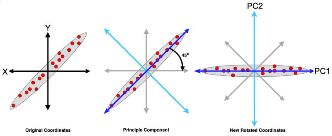
If the two components are uncorrelated, their directions should be orthogonal (image below). This image is based on simulated data with 2 predictors. Notice the direction of the components; as expected, they are orthogonal. This suggests the correlation b/w these components is zero.

The \(W\) are the matrix formed by creating a matrix with the eigen vecotrs of the correlation matrix (discussed below).
All succeeding principal component follows a similar concept, i.e., they capture the remaining variation without being correlated with the previous component. In general, for \(n \times p\) dimensional data, \(\text{min}(n-1, p)\) principal component can be constructed.
The directions of these components are identified unsupervised; i.e., the response variable \(Y\) is not used to determine the component direction. Therefore, it is an unsupervised approach.
How PCA works
- PCA is based on the idea that many real-world data sets are high-dimensional, but that most of the information in the data is contained in a relatively small number of dimensions. This means that we can often reduce the dimensionality of the data without losing much information.
- To do this, PCA first calculates the covariance matrix of the data. The covariance matrix is a square matrix that shows how each pair of variables are correlated with each other.
- Next, PCA calculates the eigenvectors and eigenvalues of the covariance matrix. The eigenvectors are the directions in which the data varies the most, and the eigenvalues are the magnitudes of the variances along those directions.
- The principal components are then formed by taking linear combinations of the original variables, where the coefficients are the corresponding eigenvectors. The first principal component is the direction of greatest variance, the second principal component is the direction of second greatest variance that is orthogonal to the first principal component, and so on.
Steps of doing the PCA
Principal Component Analysis (PCA) is a dimensionality reduction technique commonly used in data analysis and machine learning. It helps uncover the underlying structure in high-dimensional datasets by transforming the data into a new coordinate system, where the axes are aligned with the directions of maximum variance.
- Centering the Data:The first step in PCA is to standardize the data. This means subtracting the mean from each variable and then dividing by the standard deviation. This ensures that all of the variables are on the same scale and that they have a mean of zero and a standard deviation of one. This ensures that the data is centered around the origin. $$X_c = X- \bar{X}$$ where:
- \(\bar{X}\) is the mean of each feature from the corresponding values.
- Computing the Covariance Matrix: The covariance matrix is a square matrix that measures the correlation between each pair of variables. The covariance between two variables is equal to the average of the product of the deviations from the mean for those two variables. $$C(x, y) = \frac{X_c^T \cdot X_c}{m-1}$$ where:
- \(X_c^T\): Transpose of the centered data matrix \(X_c\). This operation swaps the rows and columns of \(X_c\).
- \(X_c^T\cdot X_c\): Matrix multiplication of the transposed centered data \(X_c^T\) with the original centered data \(X_c\). This results in a square matrix with dimensions \(n\times n\).
- \(1/(m-1)\): This scaling factor is used to normalize the covariance matrix. It's common to divide by \(m-1\) instead of \(m\) to account for the degrees of freedom in the sample. This makes the covariance matrix an unbiased estimator of the population covariance matrix.
- Eigenvalue Decomposition: The eigenvectors and eigenvalues of the covariance matrix are the directions and magnitudes of the data's variation. The eigenvectors are the columns of a matrix \(C\), and the eigenvalues are the diagonal entries of a diagonal matrix \(\Lambda\). $$C\cdot v_i = \lambda_i \cdot v_i.$$ The eigen vectors \(v_i\) is the \(i-\)th eigenvectors, \(\lambda_i\) is the \(i-\) the eigenvalues, and \(\cdot\) denotes matrix multiplication. Each eigen vectors are orthogonal to one another and form an orthogonal basis for the data. It also represent the directions of maximum varaince, and the corressponding eigenvalues indicate the magnitude of varaince along those directions.
- Sorting and Selecting Principal Components: The eigenvalues are sorted in descending order, and the corresponding eigenvectors are arranged accordingly. The principal components are selected based on the desired dimensionality reduction. If you want to reduce the data to k dimensions, you select the top k eigenvectors. More precisely, a common rule of thumb is to choose \(k\) principal components, where \(k\) is the maximum number of components that explain at least \(95\%\) of the varaince in the data.
- Project the data onto the principal components: The original data is then projected onto the selected principal components. The transformed data matrix \(Y\) is given by: $$Y = W^T \cdot X_c$$ where \(W^T\) is the transpose of matrix of eigenvectors and \(X_c\) is the matrix of the standardized data.
- Normalize the principal components: The principal components may not be normalized, which means that they may not have unit variance. To normalize the principal components, we divide each component by its standard deviation: $$Y = \frac{Y}{||Y||}$$ where:
- \(Y\) is the matrix of normalized principle components,
- \(||Y||\) is the frobenius norm of the mtrix \(Y\).
- The new coordinate in \(Y\) represent the data in the principle component space. The first principal component (PC1) captures the most varaince, followd by (PC2), and so on. By choosing a subset of the principal components, you can achieve dimensionality reduction while retaining most of the information present in the original data.
Example:
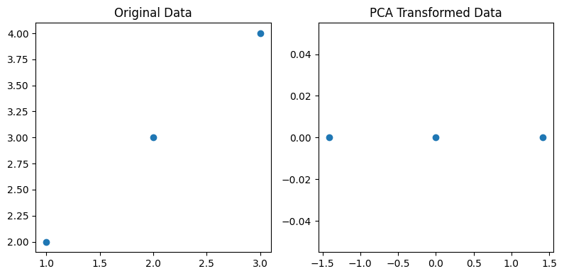
Example-1
Let's walk through a simplified mathematical example of Principal Component Analysis (PCA) using a small dataset. Consider the following 2D dataset with three observations: \begin{pmatrix} 1 & 2 \\ 2 & 3 \\ 3 & 4 \end{pmatrix}- Step 1: Centering the DataCalculate the mean of each feature and center the data by subtracting the means: $$\bar{X} = \left[\frac{1+2+3}{3} ~~~~ \frac{2+3+4}{3}\right] = [2 ~~~~ 3]$$ $$X_c = X- \bar{X} = \begin{pmatrix} -1 & -1 \\ 0 & 0 \\ 1 & 1 \end{pmatrix}$$
- Step 2: Covariance Matrix $$C = \frac{X_c^T\cdot X_c}{m-1} = \frac{1}{2} \begin{pmatrix}2 &2 \\ 2 & 2 \end{pmatrix} = \begin{pmatrix} 1 & 1 \\ 1 & 1 \end{pmatrix}$$
- Step 3: Eigenvalue Decomposition Find the eigen values \(\lambda_i\) and eigenvectors \(v_i\) of C: $$\text{det}(C - \lambda I) = 0$$ $$\text{det} \left(\begin{pmatrix} 1 - \lambda & 1 \\ 1 & 1-\lambda \end{pmatrix}\right) = 0$$ Solving for \(\lambda\) gives \(\lambda_1 =0\) and \(\lambda_2 =2\).
- For \(\lambda = 0\), the corresponding eigenvectors is \([1, -1]^T\).
- For \(\lambda = 2\), the corresponding eigenvectors is \([1, 1]^T\).
- Step 4: Sorting and Selecting Principal Components Sort the eigenvectors by their corresponding eigenvalues in descending order: $$W = \begin{pmatrix} 1 & 1 \\ -1 & 1 \end{pmatrix}$$
- Step 5: Transforming the Data Project the centered data onto the new basis: $$Y = X_c \cdot W = \begin{pmatrix} -1 & -1 \\ 0 & 0 \\ 1 & 1 \end{pmatrix} \cdot \begin{pmatrix} 1 & 1 \\ -1 & 1 \end{pmatrix} = \begin{pmatrix} -2 & 0 \\ 0 & 0 \\ 2 & 0 \end{pmatrix}$$ The transformed matrix \(Y\) representes the dataset in the principal component space.
                import numpy as np
                from sklearn.decomposition import PCA
                import matplotlib.pyplot as plt

                # Sample 2D dataset
                X = np.array([[1, 2], [2, 3], [3, 4]])

                # Step 1: Centering the Data
                mean_X = np.mean(X, axis=0)
                X_centered = X - mean_X

                # Step 2: Covariance Matrix
                cov_matrix = np.cov(X_centered, rowvar=False)

                # Step 3: Eigenvalue Decomposition
                eigenvalues, eigenvectors = np.linalg.eig(cov_matrix)

                # Step 4: Sorting and Selecting Principal Components
                sorted_indices = np.argsort(eigenvalues)[::-1]
                eigenvectors_sorted = eigenvectors[:, sorted_indices]
                # Selecting the top 2 principal components
                principal_components = eigenvectors_sorted[:, :2]

                # Step 5: Transforming the Data
                X_pca = X_centered.dot(principal_components)

                # Plotting the original and transformed data
                plt.figure(figsize=(8, 4))

                plt.subplot(1, 2, 1)
                plt.scatter(X[:, 0], X[:, 1])
                plt.title('Original Data')

                plt.subplot(1, 2, 2)
                plt.scatter(X_pca[:, 0], X_pca[:, 1])
                plt.title('PCA Transformed Data')

                plt.tight_layout()
                plt.show()
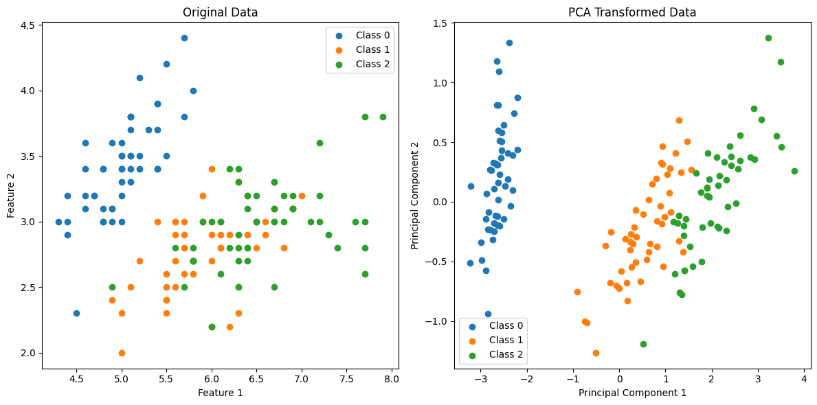
Example-2
In this example, PCA is applied to the Iris dataset, and the data is transformed to a 2D space for visualization. The reduced-dimensional representation still captures a significant amount of information, making it easier to analyze and interpret. This is just one use case; PCA is applied similarly in various machine learning scenarios for preprocessing and feature engineering.
                import numpy as np
                from sklearn.decomposition import PCA
                from sklearn.datasets import load_iris
                import matplotlib.pyplot as plt

                # Load Iris dataset as an example
                iris = load_iris()
                X = iris.data
                y = iris.target

                # Apply PCA for visualization (reduce to 2 components for simplicity)
                pca = PCA(n_components=2)
                X_pca = pca.fit_transform(X)
                # Visualize the original and PCA-transformed data side by side
                plt.figure(figsize=(12, 6))

                # Plot original data
                plt.subplot(1, 2, 1)
                for i in range(len(np.unique(y))):
                    plt.scatter(X[y == i, 0], X[y == i, 1], label=f'Class {i}')

                plt.title('Original Data')
                plt.xlabel('Feature 1')
                plt.ylabel('Feature 2')
                plt.legend()

                # Plot PCA-transformed data
                plt.subplot(1, 2, 2)
                for i in range(len(np.unique(y))):
                    plt.scatter(X_pca[y == i, 0], X_pca[y == i, 1], label=f'Class {i}')

                plt.title('PCA Transformed Data')
                plt.xlabel('Principal Component 1')
                plt.ylabel('Principal Component 2')
                plt.legend()
                plt.tight_layout()
                plt.show()
Example-3
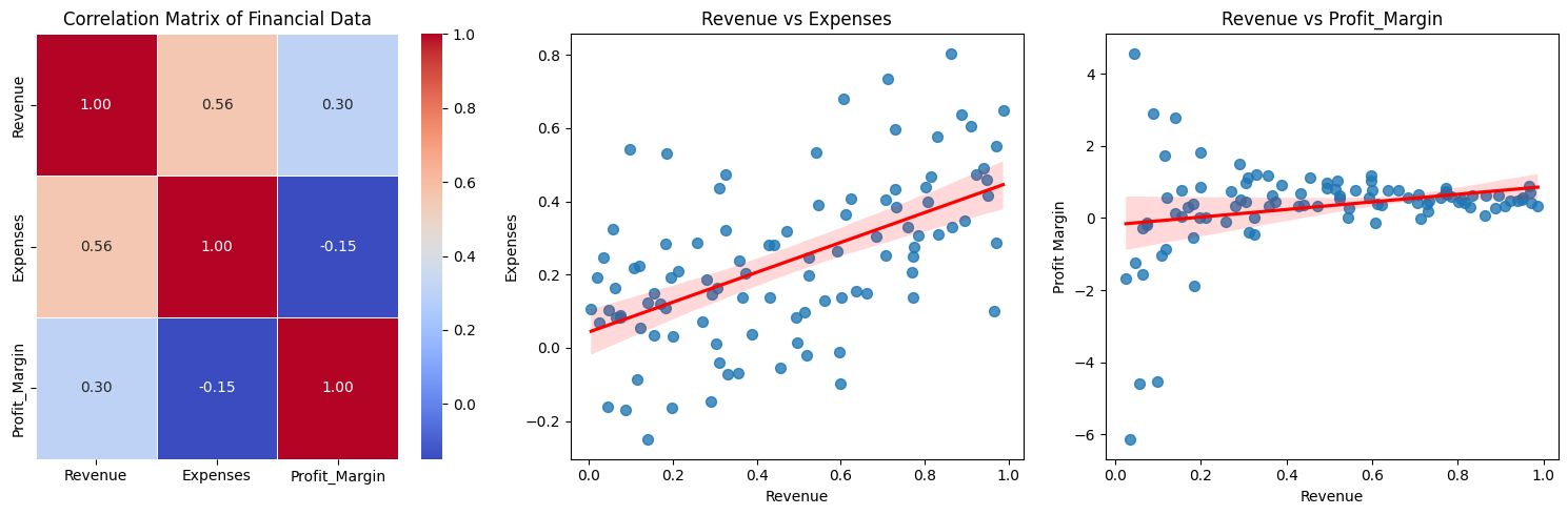
Let's consider a synthetic financial data to do the PCA analysis and find Explained variance ratio.
import numpy as np
import pandas as pd
import seaborn as sns
from sklearn.decomposition import PCA
import matplotlib.pyplot as plt
# Generate synthetic financial data
np.random.seed(42)
revenue = np.random.rand(100)
expenses = 0.5 * revenue + 0.2 * np.random.randn(100)
profit_margin = (revenue - expenses) / revenue
# Create a DataFrame
financial_df = pd.DataFrame({
'Revenue': revenue,
'Expenses': expenses,
'Profit_Margin': profit_margin
})
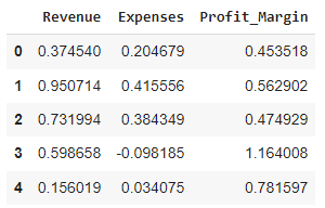
financial_df.head()
# Apply PCA
pca = PCA(n_components=2)
principal_components = pca.fit_transform(financial_df)
# Explained variance ratio
explained_variance_ratio = pca.explained_variance_ratio_
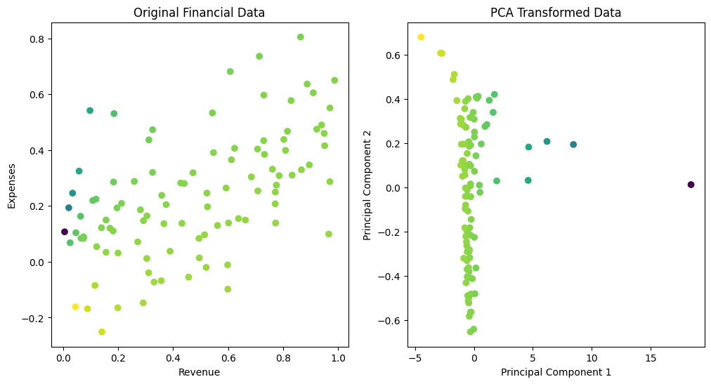
# Plotting original and PCA-transformed data
plt.figure(figsize=(12, 6))
# Original data
plt.subplot(1, 2, 1)
plt.scatter(financial_df['Revenue'], financial_df['Expenses'], c=financial_df['Profit_Margin'], cmap='viridis')
plt.title('Original Financial Data')
plt.xlabel('Revenue')
plt.ylabel('Expenses')
# PCA-transformed data
plt.subplot(1, 2, 2)
plt.scatter(principal_components[:, 0], principal_components[:, 1], c=financial_df['Profit_Margin'], cmap='viridis')
plt.title('PCA Transformed Data')
plt.xlabel('Principal Component 1')
plt.ylabel('Principal Component 2')
plt.show()
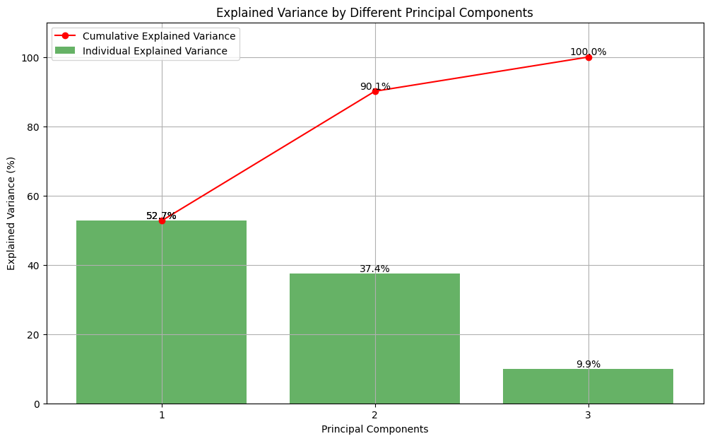
# Print explained variance ratio
print("Explained Variance Ratio:", explained_variance_ratio)
                # Extract numerical features from the DataFrame
                numerical_features = financial_df[['Revenue', 'Expenses', 'Profit_Margin']]

                # Standardize the features (optional but often recommended in PCA)
                standardized_features = (numerical_features - numerical_features.mean()) / numerical_features.std()

                # Assuming pca is the fitted PCA model
                cumulative_explained_variance = np.cumsum(pca.explained_variance_ratio_) * 100  # Convert to percentage

                # Individual explained variance as percentages
                individual_explained_variance = pca.explained_variance_ratio_ * 100

                # Create the bar plot for individual variances
                plt.figure(figsize=(12, 7))
                bar = plt.bar(range(1, len(individual_explained_variance) + 1), individual_explained_variance, alpha=0.6, color='g', label='Individual Explained Variance')

                # Create the line plot for cumulative variance
                line = plt.plot(range(1, len(cumulative_explained_variance) + 1), cumulative_explained_variance, marker='o', linestyle='-', color='r',
                                label='Cumulative Explained Variance')

                # Adding percentage values on top of bars and dots
                for i, (bar, cum_val) in enumerate(zip(bar, cumulative_explained_variance)):
                    plt.text(bar.get_x() + bar.get_width() / 2, bar.get_height(), f'{individual_explained_variance[i]:.1f}%',
                             ha='center', va='bottom')
                    plt.text(i + 1, cum_val, f'{cum_val:.1f}%', ha='center', va='bottom')

                # Aesthetics for the plot
                plt.xlabel('Principal Components')
                plt.ylabel('Explained Variance (%)')
                plt.title('Explained Variance by Different Principal Components')
                plt.xticks(range(1, len(individual_explained_variance) + 1))
                plt.legend(loc='upper left')
                plt.ylim(0, 110)  # extend y-axis limit to accommodate text labels
                plt.grid(True)
                plt.show()
Example-5 (Multivariable)
Let's now consider a multicolumn datasets and then do the PCA analysis:
# Step 1: Generate Data and Create a DataFrame
import numpy as np
import pandas as pd
import seaborn as sns
np.random.seed(42)
# Generate random data with 6 variables and more variability
data = np.random.randn(100, 10) * 5 # 100 samples, 6 variables with more variability
columns = ['Var1', 'Var2', 'Var3', 'Var4', 'Var5', 'Var6', 'Var7', 'Var8', 'Var9', 'Var10']
df = pd.DataFrame(data, columns=columns)
# Step 2: Basic Exploratory Data Analysis (EDA)
# You can explore basic statistics, correlations, etc.
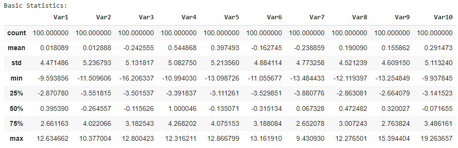
print("Basic Statistics:")
df.describe()
                # Step 3: Plot PCA Analysis
                from sklearn.decomposition import PCA
                import matplotlib.pyplot as plt

                cumulative_explained_variance = np.cumsum(pca.explained_variance_ratio_)
                individual_variance = pca.explained_variance_ratio_

                print("Cumulative Explained Variance:")
                print(cumulative_explained_variance)

                print("\nIndividual Variance Ratio:")
                print(individual_variance)
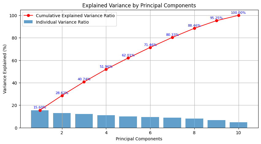
                Cumulative Explained Variance:
                [0.15598434 0.28624759 0.40740977 0.51957787 0.62005566 0.71457744
                 0.80326639 0.88455306 0.95248047 1.        ]

                Individual Variance Ratio:
                [0.15598434 0.13026324 0.12116218 0.1121681  0.10047779 0.09452177
                 0.08868896 0.08128667 0.06792741 0.04751953]
Now the PCA gave us following plot:
                # Convert cumulative explained variance to percentage
                cumulative_explained_variance_percentage = cumulative_explained_variance * 100

                # Plot the explained variance ratio with percentage values
                plt.figure(figsize=(10, 5))

                # Individual explained variance
                plt.bar(range(1, 11), individual_variance * 100, alpha=0.7, align='center', label='Individual Variance Ratio')

                # Cumulative explained variance with percentage values
                plt.plot(range(1, 11), cumulative_explained_variance_percentage, marker='o', linestyle='-', color='r', label='Cumulative Explained Variance Ratio')

                # Add percentage values to the plot
                for i, percentage in enumerate(cumulative_explained_variance_percentage):
                    plt.text(i + 1, percentage + 1, f'{percentage:.2f}%', ha='center', va='bottom', fontsize=8, color='blue')

                plt.title('Explained Variance by Principal Components')
                plt.xlabel('Principal Components')
                plt.ylabel('Variance Explained (%)')
                plt.legend()
                plt.grid(True)
                plt.show()
Description:
We can see that around 80% of the variance is explained by the first 7 principal components. The individual variance ratio for each component indicates its contribution to the overall variance.Application of PCA in machine learning
PCA is a powerful tool that can be used for a variety of machine learning tasks, including dimensionality reduction, feature extraction, and data visualization. Here are some more complex examples of how PCA can be used in machine learning:- Dimensionality reduction: One of the most common uses of PCA is for dimensionality reduction. This is when you want to reduce the number of features in a dataset while still preserving as much of the original information as possible. For example, you might be working with a dataset of images that has hundreds of features, such as the brightness, contrast, and color of each pixel. PCA can be used to reduce this number of features to a much smaller number, such as 10 or 20, while still capturing most of the important information in the images. This can make it easier to train a machine learning model on the data, and it can also make it easier to visualize the data.
- Feature extraction: Another common use of PCA is for feature extraction. This is when you want to find a new set of features that are more informative than the original features. PCA can be used to do this by identifying the directions in which the data varies the most. These directions are called principal components, and they can be used to define a new set of features. For example, you might be working with a dataset of customer data that includes features such as age, income, and spending habits. PCA can be used to identify the principal components that are most correlated with spending habits, and these can be used to define a new set of features that are more informative than the original features. This can make it easier to train a machine learning model to predict customer spending habits.
- Data visualization: PCA can also be used for data visualization. This is when you want to visualize a high-dimensional dataset in a way that is easy to understand. For example, you might be working with a dataset of financial data that includes features such as stock prices, interest rates, and economic indicators. PCA can be used to reduce the number of features in this dataset to a much smaller number, and then the data can be visualized using a scatter plot or other visualization technique. This can help you to identify patterns in the data that might not be obvious from the original dataset.
- Image compression: PCA can be used to compress images by reducing the number of pixels in the image while still preserving as much of the original information as possible. This can make it easier to store and transmit images.
- Face recognition: PCA can be used to identify faces in images. This is done by extracting the principal components of the faces in a training set, and then using these principal components to classify new faces.
- Anomaly detection: PCA can be used to detect anomalies in data. This is done by projecting the data onto the principal components, and then looking for outliers in the projected data.
- Recommendation systems: PCA can be used to recommend products or services to customers. This is done by analyzing the customer's purchase history and then using PCA to identify patterns in the data. These patterns can then be used to recommend products or services that the customer is likely to be interested in.
Practical application: Face Recognition
Principal component analysis (PCA) finds wide application in face recognition, especially in reducing the dimensionality of the data. In the context of comparing a 2D input image with a database of images to identify the best match, PCA plays a crucial role. Here, we assume that all images in the database are of identical resolution and framing, ensuring that the faces appear consistently in terms of position and scale.
In this scenario, each pixel in the images constitutes a variable, resulting in a high-dimensional problem. PCA simplifies this by identifying the principal components that capture the maximum variance in the data. By projecting the images onto a lower-dimensional subspace defined by these principal components, PCA effectively reduces the complexity of the comparison process. This allows for more efficient and accurate face recognition algorithms, even in the presence of large datasets.
In the realm of image recognition, an input image comprising \( n \) pixels is conceptualized as a point within an \( n \)-dimensional space, known as the image space. Each coordinate of this point corresponds to the intensity value of a pixel in the image, forming a row vector denoted as \( \mathbf{p}_x = (i_1, i_2, i_3, \ldots, i_n) \). This vector is constructed by concatenating the pixel values of each row in the image, resulting in a high-dimensional representation. For instance, for a moderately sized image with a resolution of 128 by 128 pixels, the dimensionality would be 16,384.

Dimension Reduction
In the context of image recognition, dimension reduction refers to the process of reducing the number of variables (or features) used to represent an image while preserving the essential information required for the task at hand. This reduction in dimensionality helps alleviate the computational burden associated with processing high-dimensional data and can also mitigate issues such as overfitting.
In the abaove image recognization example, where each pixel in an image represents a variable, dimension reduction is necessary due to the high correlation among pixels. For instance, in images with uniform backgrounds, adjacent pixels exhibit high correlation, leading to redundant information. By reducing the dimensionality of the image space, we aim to retain the most significant features while discarding redundant or less informative ones.
There are following main dimesnion reduction methods used:
- Principal component analysis (PCA)
- linear discriminant analysis (LDA),
- t-distributed stochastic neighbor embedding (t-SNE), and
- autoencoders.
These techniques offer various approaches to reducing dimensionality and extracting meaningful features from image data, ultimately improving the efficiency and effectiveness of image recognition algorithms.
Principal component analysis (PCA) is a commonly used technique for dimension reduction in image recognition. PCA identifies the principal components, which are orthogonal vectors that capture the maximum variance in the data. By projecting the data onto a lower-dimensional subspace defined by these principal components, PCA effectively reduces the dimensionality of the image space while preserving the most relevant information.
Let's consider an application where we have N images each with \(n\) pixels. We can write our entire data set as \(N\times n\) data matrix \(D\). Each row of \(D\) represents one image of our dataset. For example we may have:
\[ D = \begin{bmatrix} 150 & 152 & \dots & 254 & 255 & \dots & 252 \\ 131 & 133 & \dots & 221 & 223 & \dots & 241 \\ \vdots & \vdots & \ddots & \vdots & \vdots & \ddots & \vdots \\ \vdots & \vdots & \ddots & \vdots & \vdots & \ddots & \vdots \\ 144 & 171 & \dots & 244 & 245 & \dots & 223 \\ \end{bmatrix}_{N\times n} \]The initial stage of PCA involves shifting the origin to the mean of the data. In this context, we accomplish this by computing the mean image, denoted as \( \mu \), through the averaging of the columns of matrix \( D \). Subsequently, we subtract this mean image from every image in the dataset (i.e., each row of \( D \)) to generate the mean-centered data vector, denoted as \( U \). Suppose the mean-centered image is represented as:
$$\left[120~~~~140~~~~ ...~~~~ 230 ~~~~ 230 ~~ ... ~~ 240 \right]$$ Then we have that: \[ U = \begin{bmatrix} 30 & 12 & \dots & 24 & 25 & \dots & 12 \\ 11 & -7 & \dots & -9 & -7 & \dots & 1 \\ \vdots & \vdots & \ddots & \vdots & \vdots & \ddots & \vdots \\ \vdots & \vdots & \ddots & \vdots & \vdots & \ddots & \vdots \\ 24 & 31 & \dots & 14 & 15 & \dots & -17 \\ \end{bmatrix}_{N\times n} \]It is very easy to compute the covariance matrix from the mean centered data matrix. It is just
$$\sum = \frac{U^T U}{ N-1}$$ and has dimesnion \(n\times n\). We now calculate the eighenvectors and eigenvalues of \(\sum\) using the standard technique outlined above. That is to say we solve for \(\Phi\) and \(\Lambda\) that satisfy: $$\sum = \Phi \Lambda \Phi^T.$$ If we normalize the eigenvectors, then the system of vectors \(\Phi\) forms an orthogonal basis, that is to say:For all \( \phi_i, \phi_j \in \Phi \), we have:
\[ \phi_i \cdot \phi_j = \begin{cases} 1 & \text{if } i = j \\ 0 & \text{if } i \neq j \end{cases} \]It is in effect an axis system in which we we can represent our data in a compact form. We can achieve size reduction by choosing to represent our data we fewer dimensions. Normally we choose to use the set of \(m (m\leq n)\) eigenvectors of \(\sum\) which have the \(m\) largest eigenvalues. Typically for face recognization system \(m\) will be quite small (around 20-50 in number). We can compose these in an \(n\times m\) matrix:
$$\Phi_{\text{PCA}} = \left[\phi_1, \phi_2, ..., \phi_m \right]$$ which perfroms the PCA projection. FOr any given image \(p_x = (i_1, i_2, i_3, ... i_n)\) we can find a corresponding point in the PCA space by computing $$p_\phi = (p_x - \mu_x) \cdot \Phi_{\text{PCA}}$$ The \(m\)-dimension vector \(p_\phi\) is all we need to represent the image. We have achieved a massive reduction in data size since typically \(n\) will be least 16K and \(m\) as small as 20. We can store all our data base images in the PCA space and can easily search the data base to find the closest match to a test image. We can also reconstruct any image with the inverse transform: $$p_x =p_\phi \cdot \Phi_{\text{PCA}}^T +\mu_x$$It can be shown that choosing the m eigenvectors of \(\sum\) that have the largest eigenvalues minimises the mean square reconstruction error over all choices of m orthonormal bases.
Clearly we would like \(m\) to be as small as possible compatible with accurate recognition and reconstruction, but this problem is data dependent. We can make a decision on the basis of the amount of the total variance accounted for by the \(m\) principal components that we have chosen. This can be assessed by looking at the eigenvalues. Let the sum of all the \(n\) eigenvalues be written: \(\sum_{j=1}^n = \lambda_j\) (the \(\sum\) denoting summation in this case, not co-variance). We can express the percentage of the variance accounted for the \(i^{th}\) eigenvector as:
$$r_i = 100 \frac{\lambda_i}{\sum_{j=1}^n \lambda_j}$$We can select the value of \( m \) based on a heuristic condition that depends on the specific application. For instance, one approach could involve ensuring that we capture a minimum percentage of the total variance, such as 95%, by satisfying the condition \( \sum_{j=1}^{m} r_j \geq 95 \). Alternatively, we might discard eigenvectors whose corresponding eigenvalues contribute less than 1% to the total variance. However, there isn't a universally agreed-upon rule for determining the appropriate number of eigenvectors to retain.
References
- Google colab notebook with all the codes.
- My Github repository on machine learning Fundamentals and projects
- Nice explanation on PCA.
- Principal components analysis and exploratory and confirmatory factor analysis, Bryant, F. B., & Yarnold, P. R. (1995)In L. G. Grimm & P. R. Yarnold (Eds.), Reading and understanding multivariate analysis. Washington, DC: American Psychological Association.
- Multivariate data analysis with readings (4th ed.). Hair, J. F., Jr., Anderson, R. E., Tatham, R. L., & Black, W. C. (1995), Upper Saddle River, NJ: Prentice-Hall (a good reference book)
Some other interesting things to know:
- Visit my website on For Data, Big Data, Data-modeling, Datawarehouse, SQL, cloud-compute.
- Visit my website on Data engineering