
MCMC vs Optimal Estimation : Nonlinear Example
Some important notations and defintion:
Kernel:
$$A = \frac{\partial \hat{x}}{\partial x^{\text{true}}} = \left(K^T S_\epsilon^{-1} K + S_a^{-1}\right) K^T S_\epsilon^{-1}K$$Gain Matrix:
$$\hat{S} K^T S_\epsilon^{-1}$$ Therefore the $$\hat{x} = x_a + G (y-Kx)$$Posterior error covariance:
$$\hat{S} = \left(K^T S_\epsilon^{-1} K + S_a^{-1}\right)^{-1}$$Goal: Build a clean, self-contained mathematical example (no physics).
1. The Setup
Nonlinear forward model:
$$F(x) = x^2$$Observation:
$$y = 9.5 ~~(\text{true value is}~~ x_\text{true} = 3, ~~\text{but measurement has noise})$$Measurement noise:
$$σ_\epsilon = 0.5$$Prior:
$$x_a = 2.0, \sigma_a = 2.0$$2. Posterior
$$ P(x|y) \propto P(y|x) · P(x) = exp(−(y − F(x))^2 / 2σ_ε^2) · exp(−(x − x_a)^2 / 2σ_a^2) $$Plugging in \(F(x) = x^2\):
$$ P(x|y) \propto exp(−(9.5 − x^2)^2 / 0.5) · exp(−(x − 2)^2 / 8) $$Key point: Not Gaussian due to \(x^2\) → nonlinear model.
3. Cost Function J(x)
$$ J(x) = (9.5 − x²)² / 0.25 + (x − 2)² / 4 $$Derivative:
$$ dJ/dx = −16x(9.5 − x²) + 0.5(x − 2) = 0 $$This is a cubic equation → must solve iteratively.
4. Gauss-Newton Iteration
Linearisation: Linearisation around \(x_i\)
$$ F(x) \approx F(x_i) + K_i \, (x - x_i)\\ \text{where } \quad K_i = \left.\frac{dF}{dx}\right|_{x_i} = 2x_i ~~~~~~~~~~ \leftarrow \text{the Jacobian} $$Gauss-Newton update formula:
$$ x_{i+1} = x_a + \left( \frac{K_i^2}{\sigma_\epsilon^2} + \frac{1}{\sigma_a^2} \right)^{-1} \cdot \frac{K_i}{\sigma_\epsilon^2} \cdot \left[ y - F(x_i) + K_i (x_i - x_a) \right] $$Let's iterate numerically, starting from prior \(x_0 = 2.0\):
Iteration 1
$$ x_i = 2.0 \\ F(2.0) = 4.0 \\ K_i = 2 x_i = 4.0 \\ \text{residual} = y - F(x_i) = 9.5 -4.0 = 5.5 \\ \text{Hessian} = \frac{K^2}{\sigma_\epsilon^2} + \frac{1}{\sigma_a^2} = \frac{16}{0.25} + \frac{1}{4} = 64.25 \\ \text{rhs} = \frac{K}{\sigma_\epsilon^2} \times [\text{residual} + K(x_i - x_a)] = \frac{4}{0.35} \times [5.5 + 4\times (2-2)] =88.0 \\ x_{i+1} = x_a + \text{rhs}/\text{Hessian} = 2.0 + 88.0/64.25 = 2.0 + 1.370 = 3.370 $$Iteration 2
$$ F(3.370) = 11.357 \\ K_i = 2 \times 3.370 = 6.740 \\ \text{residual} = 9.5 - 11.357 = -1.857\\ \text{Hessian} = 6.74^2/0.25 + 0.25 = 181.8\\ \text{rhs} = 6.74/0.25 \times [-1.857 + 6.74\times(3.370-2)] = 26.96 \times [-1.857 + 9.232] = 26.96 \times 7.375 = 198.8 \\ x_{i+1} = 2.0 + 198.8/181.8 = 2.0 + 1.094 = 3.094 $$Iteration 3
$$ F(3.094) = 9.573 \\ K_i = 6.188 \\ \text{residual} = 9.5 - 9.573 = -0.073 \\ x_{i+1} ≈ 3.081 $$Iteration 4
$$ x_i = 3.080 \rightarrow x_{i+1} =3.080 \Rightarrow \text{converged} $$5. Posterior Covariance
At the solution: \(\hat{x} = 3.080\), \(K=2\times 3.080 = 6.160\) $$ S_x = (K²/σ_ε² + 1/σ_a²)⁻¹ = (151.9 + 0.25)⁻¹ = 0.00657 $$Standard deviation:
$$σ_{post} = \sqrt{0.00657} = 0.081$$Result:
$$\hat{x} = 3.080 ± 0.081$$6. Averaging Kernel
$$ A = S_x \frac{K^2}{\sigma_\epsilon^2} = 0.998 $$→ Measurement dominates, prior is weak.
\(A\approx 1.0\) means the retrieval is almost entirely driven by the measurement, not the prior. The prior $\sigma_a =2.0$ was broad, so the measurement dominates.
7. NOW See Why the Gaussian Assumption is Wrong : True Posterior Shape
OE gave us \(\hat{x} = 3.080 \pm 0.081\) -- a symmetric Gaussian.
But look at the true posteriro shape. The cost function is: $$ J(x) = \frac{(9.5 - x²)^2}{0.25} + \frac{(x − 2)^2}{4} $$ We can draw a graph for this function as: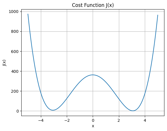
There is a second mode near \(x = -3.08\) because \(F(x) =x^2\) is symmetric. OE completely misses this -- it found the positive solution. MCMC would find both.
Also \(J(x)\) rises much faster on the right \(x> 3.08\) than on the left -- the posterior is asymmetric. OE's symmetric \(\pm 0.081\) is therefore an approximation.
Important:
- Second mode exists at x ≈ −3.08
- Posterior is asymmetric
- OE misses this completely
8. What MCMC Would Do Differently?
MCMC samples \( P(x|y) \propto \text{exp}\left(-\frac{J(x)}{2}\right)\) directly. It would reveal:- Mode 1: \(x \approx +3.08 \) (positive root)
- Mode 2: \(x \approx -3.08 \) (negative root - missed by OE!)
- Asymmetry: Longer tail on left side of each mode
9. Summary — The Two Assumptions Visualised
                TRUE POSTERIOR                                  OE APPROXIMATION
                (what MCMC finds)                               (what OE assumes)

                    │                                           │
                    │  *                                        │    *
                    │ ***   *                                   │   ***
                    │*****  **                                  │  *****
                ────┼──────────── x                         ────┼──────────── x
                -3.08  +3.08                                only +3.08

                Bimodal + asymmetric                        single Gaussian
10. Final Insight
The nonlinear model F(x) = x² causes:
- Non-Gaussian posterior -- asymmetric tails
- Multiple solutions -- two solutions OE cannot see
- Asymmetry
This is exactly what happens in real CO₂ retrieval problems when degeneracies exist.
Reference
- Fundamentals of Remote sensing
- Relevance of Electromagnetic waves in the context of earth observation
- Concept of the orbits for a satellite (non scientific discussion)
- How various teams works in close collaboration for the ground data processing?
- How raw satellite data is processed to do a level where you do your scientifc research?
- In depth understandingof the satellite data (op-of-atmosphere reflectance)
- Resolution and calibration
- Understanding how OLCI data is processed
- Transforming Energy into Imagery: How Satellite Data Becomes Stunning Views of Earth