Introduction

• Support Vector Machine (SVM) is undoubtedly one of the most popular ML algorithms used by machine learning practitioners. It is a supervised machine learning algorithm that is robust to outliers and generalizes well in many cases. However, the intuitive idea behind SVM can be a bit tricky to understand for a beginner. The name in itself is quite intimidating, Support, Vector, and Machine.
• It is used for Classification as well as Regression problems. However, primarily, it is used for Classification problems in Machine Learning.
• In this algorithm, we try to find a hyperplane that best separates the two classes. It is to be noted that, it may seems that the SVM and logisitc regression are similar. Both the algorithms try to find the best hyperplane, but the main difference is logistic regression is a probabilistic approach whereas support vector machine is based on statistical approaches.
• Now the question is which hyperplane does it select? There can be an infinite number of hyperplanes passing through a point and classifying the two classes perfectly. So, which one is the best? Well, SVM does this by finding the maximum margin between the hyperplanes that means maximum distances between the two classes.

Types of Support Vector Machine (SVM) Algorithms

Support Vector Machines (SVMs) offer various algorithms for classification and regression tasks, primarily distinguished by the types of decision boundaries they create and the techniques they employ for optimization. Here are some common types of SVM algorithms:

1. Linear SVM: This algorithm is used when the data is linearly separable. Perfectly linearly separable means that the data points can be classified into 2 classes by using a single straight line(if 2D). It aims to find the optimal hyperplane that separates the classes with the maximum margin.
2. Non-linear SVM: When the data is not linearly separable then we can use Non-Linear SVM, which means when the data points cannot be separated into 2 classes by using a straight line (if 2D) then we use some advanced techniques like kernel tricks to classify them. In most real-world applications we do not find linearly separable datapoints hence we use kernel trick to solve them.
3. Support Vector Regression (SVR): Unlike classification tasks, SVR is used for regression tasks. It aims to find the optimal hyperplane that best fits the data while minimizing the margin violations.
4. Nu-SVM: This algorithm is an extension of the traditional SVM, introducing a parameter "nu" that replaces the regularization parameter "C." It offers a more intuitive control over the number of support vectors and margin errors.
5. One-Class SVM: Primarily used for anomaly detection, this algorithm learns a decision boundary that encompasses the majority of the data points while treating the rest as outliers.
6. Sequential Minimal Optimization (SMO): SMO is an algorithm for training SVMs, particularly useful for solving large-scale optimization problems by decomposing them into smaller sub-problems.
7. Least Squares SVM (LS-SVM): This variant of SVM reformulates the optimization problem as a set of linear equations, making it computationally efficient for large-scale datasets.
8. Budgeted SVM: Designed for scenarios with limited computational resources, this algorithm dynamically selects a subset of support vectors to reduce computational complexity while maintaining classification accuracy.

Important terminologies

Here are some important terms in the context of Support Vector Machines (SVM):

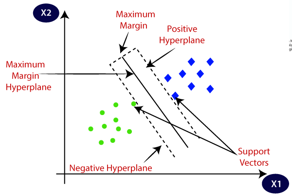
• Hyperplane: In SVM, a hyperplane is a decision boundary that separates classes in a feature space. For a binary classification problem, it's a line in 2D space, a plane in 3D space, and a higher-dimensional surface in higher dimensions.
• Margin: The margin is the distance between the hyperplane and the nearest data points of each class. SVM aims to maximize this margin, as it represents the separation between classes. Maximizing the margin helps improve generalization and reduces the risk of overfitting.
• Support Vectors: These are the data points that lie closest to the decision boundary (hyperplane). They determine the position and orientation of the hyperplane and are crucial in defining the margin. Only these points influence the construction of the hyperplane; hence, they are called support vectors.
• Kernel Trick: SVMs can efficiently handle non-linear decision boundaries by using kernel functions. The kernel trick involves implicitly mapping the input features into a higher-dimensional space, where the classes are more likely to be separable. Common kernel functions include linear, polynomial, radial basis function (RBF), and sigmoid.
• Regularization Parameter (C): The regularization parameter (C) controls the trade-off between maximizing the margin and minimizing the classification error. A smaller C value leads to a larger margin but may result in misclassification of some training examples (soft margin). Conversely, a larger C value allows more training examples to be correctly classified but may lead to a smaller margin (hard margin). Proper tuning of C is crucial to prevent overfitting.
• Kernel Parameters: For kernelized SVMs, there are additional parameters to tune, such as gamma (\(\gamma\)) for RBF kernel and degree for polynomial kernel. These parameters control the flexibility of the decision boundary. Proper selection of kernel parameters is essential for achieving good performance and avoiding overfitting.
• Dual Problem: The optimization problem in SVM can be reformulated into its dual form, which involves maximizing a function subject to constraints. Solving the dual problem is often more computationally efficient, especially when using kernel functions.
• Nu Parameter: In Nu-SVM, the nu parameter replaces the C parameter and controls the upper bound on the fraction of margin errors and support vectors. It offers a more intuitive way to adjust the model complexity.

Useful application of SVM

Support Vector Machines (SVMs) are versatile algorithms that find applications in various fields due to their ability to handle both linear and non-linear classification problems efficiently. Here are some common applications of SVM:

• Image Classification: SVMs are widely used in image classification tasks, such as identifying objects or scenes within images. They can efficiently handle high-dimensional feature spaces and are robust to noise.
• Text Classification: SVMs are employed in text classification tasks, such as spam email detection, sentiment analysis, and document categorization. They can effectively classify text data represented as high-dimensional feature vectors.
• Handwriting Recognition: SVMs are used in handwriting recognition systems, where they classify handwritten characters or digits into different classes. They can handle complex patterns and variations in handwriting styles.
• Biomedical Applications: SVMs find applications in various biomedical tasks, including disease diagnosis, protein classification, and gene expression analysis. They can analyze high-dimensional biomedical data and identify patterns indicative of specific conditions.
• Financial Forecasting: SVMs are utilized in financial forecasting tasks, such as stock price prediction, credit scoring, and fraud detection. They can analyze historical financial data and identify patterns to make predictions about future trends or events.
• Bioinformatics: SVMs are applied in bioinformatics for tasks such as protein structure prediction, DNA sequence analysis, and protein-protein interaction prediction. They can handle large-scale biological data and extract meaningful patterns.
• Remote Sensing: SVMs are used in remote sensing applications, such as land cover classification, crop classification, and environmental monitoring. They can analyze satellite imagery and classify different land cover types accurately.
• Face Detection: SVMs are employed in face detection systems, where they classify image regions as containing faces or background. They can effectively distinguish between facial features and background clutter.
• Medical Diagnosis: SVMs are used in medical diagnosis tasks, such as cancer detection, disease prognosis, and patient outcome prediction. They can analyze medical data from various sources and assist healthcare professionals in decision-making.
• Anomaly Detection: SVMs are utilized in anomaly detection systems to identify unusual or unexpected patterns in data. They can detect outliers or anomalies that deviate significantly from normal behavior.

Pros

1. Effective in High-Dimensional Spaces: SVMs perform well in high-dimensional spaces, making them suitable for tasks involving a large number of features, such as image classification and text categorization.
2. Robust to Overfitting: SVMs are less prone to overfitting compared to other algorithms like decision trees. By maximizing the margin between classes, SVMs generalize well to unseen data.
3. Versatile Kernel Functions: SVMs can handle non-linear decision boundaries using various kernel functions (e.g., polynomial, radial basis function), allowing them to capture complex relationships in the data.
4. Works Well with Small Datasets: SVMs can perform well even with relatively small datasets, as they focus on the points closest to the decision boundary (support vectors) rather than the entire dataset.
5. Global Optimization: SVMs use convex optimization techniques to find the optimal hyperplane, ensuring that the solution is globally optimal and not affected by local minima.
6. Regularization Parameter: SVMs offer a regularization parameter (C) that allows users to control the trade-off between maximizing the margin and minimizing classification errors, providing flexibility in model tuning.

Cons

1. Sensitivity to Parameter Tuning: SVMs require careful selection of parameters, such as the choice of kernel function and regularization parameter. Improper parameter tuning can lead to suboptimal performance.
2. Computationally Intensive: Training an SVM can be computationally intensive, especially for large datasets. The training time and memory requirements increase significantly with the number of data points.
3. Limited Interpretability: The decision boundary produced by SVMs may be difficult to interpret, particularly when using complex kernel functions or in high-dimensional spaces. This limits the insight into the underlying relationships in the data.
4. Memory Usage: SVMs require storing all support vectors in memory, which can become impractical for very large datasets with numerous support vectors, leading to high memory usage.
5. Binary Classification: SVMs are inherently binary classifiers and need additional techniques (e.g., one-vs-all) to handle multi-class classification problems, which can increase complexity.
6. Sensitive to Noise: SVMs can be sensitive to noise in the training data, as outliers or mislabeled points near the decision boundary may significantly affect the model's performance.

Mathematical intuition behind the Support Vector Machine

Support-vector-machine explanation: 2D

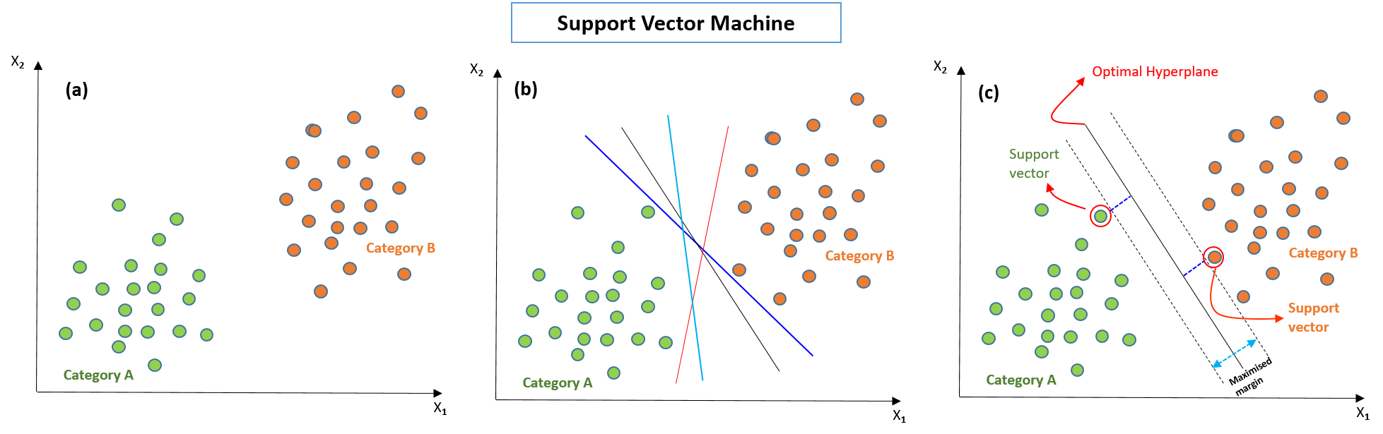
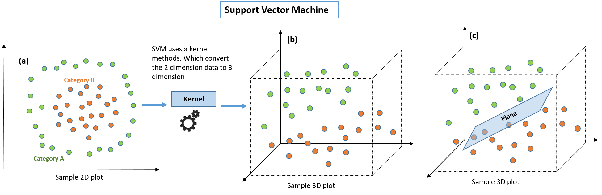
Imagine you have a scatter plot where the green points represent one class and the orange points represent another class. To separate these two classes, an SVM seeks to find the best-fitting line or plane (hyperplane) that maximizes the margin between the two classes. We can find the best line by computing the maximum margin from equidistant support vectors.

Let's understand it in detail. We want to classify that the new data point as either green or orange. To classify these points, we can have many decision boundaries, but the question is which is the best and how do we find it? The best hyperplane is that plane that has the maximum distance from both the classes, and this is the main aim of SVM. This is done by finding different hyperplanes which classify the labels in the best way then it will choose the one which is farthest from the data points or the one which has a maximum margin.

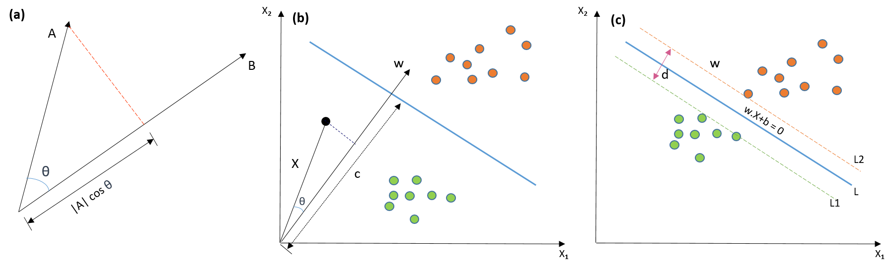
Let's understand first what is dot product of vectors. The dot product can be defined as the projection of one vector along with another, multiply by the product of another vector and is defined as \(\vec{A} \cdot \vec{B} = |A| \cos \theta |B| \), where \(|A| \cos \theta\) is the projection of \(\vec{A}\) on \(\vec{B}\). In SVM, we just need the projection of \(\vec{A}\) not the magnitude of \(\vec{B}\). Instead we take \(\vec{A} \cdot \vec{B} = |A| \cos \theta \times ~(\text{unit vector of } \vec{B})\) as to get the projection, we can just take the unit vector of \(\vec{B}\) because it will be in the direction of \(\vec{B}\) but its magnitude will be 1. Now let's consider image (b) in the above figure where we consider a random data point in black and corresponding vector \(\vec{X}\). We aim to determine if a point lies to the right (positive) or left (negative) side of the separating line (plane). This is done by computing the dot product of the vector onto the perpendicular line to the boundary separating the two sets of data points (green and orange). Here \(c\) is the distance of the light blue separing line from the origin. Now following three conditions may arise:

Here the dot product of the two vectors (where \(\vec{w}\) is a unit vector perpendicular to the decision boundary), gives the distance of vector X from the decision boundary and there may be infinte points on the boundary to measure the distance from. We simply take perpendicular and use it as a reference and then take projections of all the other data points on this perpendicular vector and then compare the distance. In SVM we also have a concept of margin. We can rewrite the equation \(\vec{X} \cdot \vec{w} -c \geq 0 \Rightarrow \vec{X} \cdot \vec{w} +b \geq 0 \), where we just replaced \(-c\) with the \(b\).

Therefore, we have

If the value of \(\vec{X}\cdot \vec{w} +b>0\) then we can say it is a positive point otherwise it is a negative point. Now we need \((w,b)\) such that the margin has a maximum distance. Let’s say this distance is '\(d\)'. To calculate \(d\), we need the equation of the two lines L1, and L2. We want our plane to have equal distance from both the classes that means L should pass through the center of L1 and L2 that’s why we take magnitude equal. For mathematical convience, we consider the equations of the two lines \(\vec{X}\cdot \vec{w} +b =1\) and \(\vec{X}\cdot \vec{w} +b = -1\). Another reason, why choose 1, is if we multiply the equation of hyperplane with a factor greater than 1 then the parallel lines will shrink and if we multiply with a factor less than 1, they expand. We can now say that these lines will move as we do changes in \((w,b)\) and this is how this gets optimized. But what is the optimization function? Let’s calculate it. We know that the aim of SVM is to maximize this margin that means distance \((d)\). But there are few constraints for this distance \((d)\). Let’s look at what these constraints are.

Optimization function and its constrainsts

1. Hard Margin SVM: Since, for orange points \(\vec{w}\cdot \vec{X} +b \leq -1\) and for green points \(\vec{w}\cdot \vec{X} +b \geq 1\) i.e. negative classes have \(y = -1\) and positive classes have \(y = 1\). We can say that for everypoint to be correctly classfied, above two condition can be combined as: $$y_i(\vec{w}\cdot \vec{X}+b)\geq 1$$
   • Suppose a green point is correctly classfied that means it will follow \(\vec{X}\cdot \vec{w} +b >=1\), if we multiply this with \(y=1\) we get this same equation mentioned above.
   • Similarly, if we do this with a orange point with \(y=-1\) we will again get this equation. Hence, we can say that we need to maximize (d) such that this constraint holds true.

   

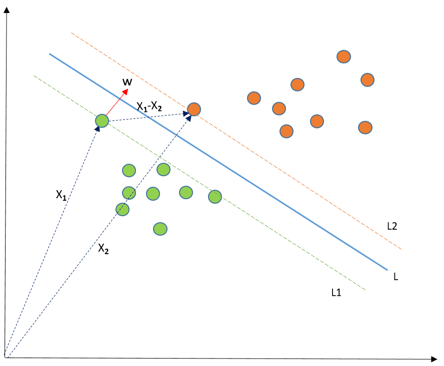
   Now we can consider two support vectors, one from negative class and second from the positive class. The distance between the two vectors \(\vec{X}_1\) and \(\vec{X}_2\) will be \(\vec{X}_2 - \vec{X}_1\). What we need is, the shortest distance between these two points which can be found using a trick we used in the dot product. We take a vector \(\vec{w}\) perpendicular to the hyperplane and then find the projection of \(\vec{X}_2\) will be \(\vec{X}_2 - \vec{X}_1\) vector on \(\vec{w}\), where \(\vec{w}\) is the unit vector. Therefore the projection of avector on another vector is: $$(\vec{X}_2 -\vec{X}_1)\cdot \frac{\vec{w}}{\|\vec{w}\|} \Rightarrow \frac{\vec{X}_2 \cdot \vec{w} -\vec{X}_1 \cdot \vec{w} }{\|\vec{w}\|}.$$ Since the two vectors \(X_2\) and \(X_1\) are support vectors and they lie on the hyperplane, we can write: \(y_i (\vec{w}\cdot \vec{X}+b) = 1\), i.e \(1\times (\vec{w}\cdot \vec{X}+b) = 1 \Rightarrow \vec{w}\cdot \vec{X}_1 =1- b\) for positive point (\(y=1\)) and \(-1 \times (\vec{w}\cdot \vec{X}+b) = 1 \Rightarrow \vec{w}\cdot \vec{X}_1 = - 1- b\). Yherefore, substituing the two value in above equations: $$\frac{\vec{X}_2 \cdot \vec{w} -\vec{X}_1 \cdot \vec{w} }{\|\vec{w}\|} = \frac{(1-b) - (-1-b)}{\|\vec{w}\|} =\frac{2}{\|\vec{w}\|} = d.$$

   Hence the equation which we have to maximize in the context of finding the maximum margin separating hyperplane is:

   $$\text{argmax}_{(\vec{w}^*, b^*)} \left(\frac{2}{\|\vec{w}\|}\right) \Rightarrow \text{such that} ~~~ y_i \left( \vec{w}\cdot \vec{X}+b\right)\geq 1.$$

   This type of SVM is known as Hard Margin SVM. It is to be noted that, in reality there is hardly any case we get perfectly linearly separable data and hence we fail to use this condition we proved here.

2. Soft Margin SVM: In a traditional SVM, we aim to find a hyperplane that separates the data into two classes with the largest margin possible. However, in real-world scenarios, the data might not be linearly separable, or there could be outliers that affect the decision boundary. The Soft Margin SVM addresses these issues by allowing for some misclassifications and incorporating a penalty term for them. Mathematically, let's start with the optimization problem for the Soft Margin SVM. Given training data \((x_1, y_1),(x_2, y_2), (x_n, y_n)\), where \(x_i \in \mathbb{R}^d\) is the input feature vector and \(y_i \in \{-1, 1\}\) is the corresponding class label, the Soft Margin SVM aims to find the hyperplane represented by \(\mathbf{w} \cdot \mathbf{x} + b = 0\) that maximizes the margin while allowing for some misclassifications.
   📌 Note: Here it is to be noted here that we took argmin instead of argmax compared to the Hard Margin SVM. We know that \(\text{max}[f(x)]\) can also be written as \(\min[1/f(x)]\), it is common practice to minimize a cost function for optimization problems; therefore, we can invert the function argmax function to argmin.
   \[ \text{argmin}_{\mathbf{w}, b, \boldsymbol{\xi}} \left( \frac{1}{2}||\mathbf{w}||^2 + C\sum_{i=1}^{n} \xi_i \right) \]

   subject to the constrainsts:

   $$y_i(\mathbf{w} \cdot \mathbf{x}_i + b) \geq 1 - \xi_i \quad \text{and} \quad \xi_i \geq 0, \quad \forall i.$$
   • Here, \(C > 0\) is the regularization parameter that controls the trade-off between maximizing the margin and minimizing the classification errors. A larger \(C\) value penalizes misclassifications more heavily, leading to a narrower margin but potentially better classification accuracy. It is a hyperparameter and we find the optimal value of \(C\) using GridsearchCV and cross-validation.
   • The term \(\frac{1}{2}||\mathbf{w}||^2\) represents the margin maximization objective, aiming to maximize the margin between the support vectors (data points closest to the decision boundary) of different classes.
   • The term \(C\sum_{i=1}^{n} \xi_i\) serves as the regularization term, penalizing misclassifications. By minimizing this term, we encourage the SVM to find a balance between maximizing the margin and minimizing classification errors.

   In summary, the Soft Margin SVM introduces slack variables to handle misclassifications and incorporates a regularization parameter to control the trade-off between margin maximization and error minimization. This approach allows the SVM to generalize better to real-world datasets with noise or non-linearly separable classes.

So in summary when using an SVM to classify data points into different classes:

• Support vectors are chosen as the data points closest to the separating hyperplane.
• The margin, or the distance between the support vectors and the hyperplane, is maximized to ensure robust classification.
• Each data point's influence on determining the hyperplane's position is weighted based on its proximity to the hyperplane.

Classification problem with higher dimension data

The data set shown below in Image-(a) has no clear linear separation between the two classes. In machine learning parlance, we would say that these are not linearly separable. How can we get the support vector machine to work on such data?

Since we can't separate it into two classes using a line, we need to transform it into a higher dimension by employing a kernel function to the data set. A higher dimension enables us to clearly separate the two groups with a plane. Here, we can draw some planes between the green dots and the orange dots — with the end goal of maximizing the margin. If we let R=the number of dimensions, the kernel function will convert a two-dimensional space (R2) to a three-dimensional space (R3). Once the data is separated into three dimensions, we can apply SVM and separate the two groups using a two-dimensional plane. For a higher dimension, we would have to use higher diemntsional curve.

Kernel Functions

Kernel functions play a fundamental role in Support Vector Machines (SVMs), enabling them to handle non-linear relationships between features and find complex decision boundaries. Let's delve into a detailed explanation of kernel functions:

Purpose of Kernel Functions

Kernel functions are mathematical transformations applied to input data in SVMs. Their primary purpose is to map the original input space into a higher-dimensional feature space, where the classes may be more easily separable by a hyperplane. By transforming the data into a higher-dimensional space, kernel functions enable SVMs to capture non-linear relationships and complex patterns in the data. A kernel function, denoted as \(K(\textbf{x}, \textbf{x}')\), takes two input vectors \(\textbf{x}\) and \(\textbf{x}'\) and computes a measure of similarity or distance between them. This measure is often represented as the dot product of the transformed feature vectors in the higher-dimensional space.

Types of Kernel Functions

There are several types of kernel functions commonly used in SVMs. For the input vectors \(\textbf{x}\) and \(\textbf{x}'\):

1. Linear Kernel \(K_{\text{linear}}(\textbf{x},\textbf{x}')\): This is the simplest kernel function, where the dot product of the input vectors is computed directly in the original feature space. It is suitable for linearly separable data. $$K_{\text{linear}}(\textbf{x}, \textbf{x}') = \textbf{x}^T \textbf{x}'$$ here \(\textbf{x}^T\) represents the transpose of vector \(\textbf{x}\), and \(\textbf{x}'\) is another vector.
   • Interpretation: The linear kernel measures the similarity between two vectors by taking into account the alignment of their features. It computes the weighted sum of the products of corresponding features in the input vectors.
   • Features: In the original feature space, each input vector \(\textbf{x}\) is represented by a set of features. The dot product \(\textbf{x}^T \textbf{x}'\) calculates the sum of the products of corresponding features in vector \(\textbf{x}\) and \(\textbf{x}'\), effectively measuring their similalrity.
   • Linear Separation: The linear kernel is suitable for linearly separable data, where a straight line (or hyperplane in higher dimensions) can effectively separate the classes. It works well when the decision boundary between classes can be represented by a linear equation.
   • Advantages:
     • Simplicity: The linear kernel is straightforward and computationally efficient.
     • Interpretability: The decision boundary learned by SVM with a linear kernel can be easily interpreted as a linear combination of input features.
   • Limitations:
     • Limited Complexity: The linear kernel may not capture complex relationships between features and classes, making it less suitable for datasets with non-linear separability.
     • Performance on Non-linear Data: In cases where the data is not linearly separable, the linear kernel may lead to suboptimal classification performance.
   • Applications:
     • Text Classification: Linear kernels are commonly used in text classification tasks where the feature space is often high-dimensional.
     • Linear Regression: Linear kernels can be applied in linear regression problems to model relationships between input features and target variables.
   • Example:Let's consider a simple example with two input vectors \(\textbf{x}\) and \(\textbf{x}'\) represented by two-dimensional feature vectors. The linear kernel computes the dot product of these vectors directly in the original feature space. Suppose we have two input vectors $$x = \begin{pmatrix} x_1 \\ x_2 \end{pmatrix}$$ and $$x' = \begin{pmatrix} x'_1 \\ x'_2 \end{pmatrix}$$

     The linear Kernel between the two vectors is computed as:

     $$K_{\text{linear}}(\textbf{x}, \textbf{x}') = \textbf{x}^T \textbf{x} =\begin{pmatrix} x_1 & x_2 \end{pmatrix} \begin{pmatrix} x'_1 \\ x'_2 \end{pmatrix} = x_1 x_1'+x_2 x_2'$$ This equation represents the similarity between the two input vectors \(\textbf{x}\) and \(\textbf{x}'\) based on the alignment of their features. The larger the value of the Kernel \(K_{\text{linear}}(\textbf{x}, \textbf{x}')\), the more similar the vectors \(\textbf{x}\) and \(\textbf{x}'\) are considered to be. For example two vectors: $$x = \begin{pmatrix} 2 \\ 3 \end{pmatrix}$$ and $$x' = \begin{pmatrix} 4 \\ 1 \end{pmatrix}$$ Kernel \(K_{\text{linear}}(\textbf{x}, \textbf{x}') = 11\) indicating a relatively high similalrity between the two inputs vectors.
2. Polynomial Kernel \(K_{\text{poly}}(\textbf{x},\textbf{x}')\): The Polynomial Kernel is a type of kernel function used in Support Vector Machines (SVMs) to handle non-linear relationships between features. It transforms the input data into a higher-dimensional space, where it may be easier to find a separating hyperplane. The polynomial kernel raises the dot product of the input vectors to a certain power \(d\), allowing SVMs to capture polynomial decision boundaries. It is defined as $$K_{\text{poly}}(\textbf{x},\textbf{x}') = \left(\textbf{x}\cdot \textbf{x}'+c\right)^d,$$ where \(c\) is a constant and \(d\) is the degree of the polynomial.
   • Role of Parameters:
     • Degree \((d)\): The degree parameter determines the degree of the polynomial transformation applied to the input data. Higher values of \(d\) result in more complex decision boundaries.
     • Constant \((c)\):The constant term acts as a bias and helps control the influence of lower-degree polynomials. It shifts the decision boundary away from the origin in the feature space.
   • Kernel Properties:
     • Linearity: Despite its name, the Polynomial Kernel is capable of capturing non-linear relationships between features. By raising the dot product of the input vectors to a higher power, the kernel can represent complex decision boundaries.
     • Computational Complexity: The computational complexity of the Polynomial Kernel depends on the degree parameter \(d\). Higher values of \(d\) increase the computational cost, as they require computing higher-order polynomials.
   • Choice of Parameters:
     • Degree \((d)\): The degree parameter should be chosen based on the complexity of the data and the desired level of model flexibility. Higher values of \(d\) may lead to overfitting if the data is not complex enough to warrant such a high-degree polynomial.
     • Constant Term \((c)\): The constant term \(c\) can be set empirically or through cross-validation. It helps adjust the bias of the model and fine-tune the decision boundary.
   • Example Application: The Polynomial Kernel is commonly used in SVMs for tasks such as image classification, text classification, and pattern recognition. It is effective in capturing non-linear relationships between features and constructing complex decision boundaries in high-dimensional feature spaces.

   In summary, the Polynomial Kernel is a versatile kernel function that allows SVMs to handle non-linear relationships between features by transforming the input data into a higher-dimensional space. It offers flexibility in capturing complex patterns and can be customized through parameters like degree and constant term to suit the characteristics of the data.

3. Radial Basis Function (RBF) Kernel \(K_{\text{RBF}}(\textbf{x}, \textbf{x}')\): The Radial Basis Function (RBF) kernel, also known as the Gaussian kernel, is a popular choice in Support Vector Machines (SVMs) for its ability to capture complex non-linear relationships between data points. The RBF kernel computes the similarity between two input vectors \(\textbf{x}\) and \(\textbf{x}'\) based on the Euclidean distance between them in the input space. Mathematically, the RBF kernel is defined as: $$K_{\text{RBF}}(\textbf{x}, \textbf{x}') = \exp\left(-\gamma \|\textbf{x} - \textbf{x}'\|^2\right)$$

   Here, \(\gamma>0\) is a parameter controlling the kernel's width, and \(\|\textbf{x}-\textbf{x}'\|\) represents the Euclidean distance between vectors \(\textbf{x}\) and \(\textbf{x}'\).

   • Interpretation:
     • The RBF kernel measures the similarity or closeness between two data points based on their distance in the input space.
     • When \(\textbf{x}\) and \(\textbf{x}'\) are close to each other, their Euclidean distance \(\|\textbf{x}-\textbf{x}'\|\) is small, resulting in a high similalrity value.
     • Conversely, when \(\textbf{x}\) and \(\textbf{x}'\) are far apart, their distance increases, leading to a lower similalrity value.
     • The paramter \(\gamma\) controls the kernel's width, determing how quickly the similalrity decays as the distance between points increases. A smaller \(\gamma\) results in a broder kernel, capturing more global relationships. while a larger \(\gamma\) focuses on local relationships.
   • Effect on SVM Decision Boundary:
     • In SVMs, the RBF kernel allows for the construction of non-linear decision boundaries that can adapt to complex data distributions.
     • By mapping the input data into a higher-dimensional feature space implicitly, the RBF kernel transforms the data in a way that enables SVMs to find optimal separating hyperplanes even for non-linearly separable data.
   • Choice of \(\gamma\):
     • The choice of the \(\gamma\) parameter is critical in determining the behavior of the RBF kernel.
     • A smaller \(\gamma\) value results in a smoother decision boundary, capturing broader patterns in the data but potentially leading to underfitting.
     • Conversely, a larger \(\gamma\) value creates a more complex decision boundary, capturing finer details in the data but increasing the risk of overfitting.
   • Application:
     • The RBF kernel is widely used in SVMs for various classification tasks, including image recognition, text classification, and bioinformatics.
     • Its flexibility in capturing non-linear relationships makes it suitable for datasets with complex structures and intricate patterns.

   In summary, the Radial Basis Function (RBF) kernel is a powerful tool in SVMs for capturing non-linear relationships between data points. Its ability to adapt to complex data distributions and construct flexible decision boundaries makes it a popular choice for a wide range of classification tasks.

4. Sigmoid Kernel: The sigmoid kernel computes the similarity between two vectors using the hyperbolic tangent function: $$K_{\text{sigmoid}}(\textbf{x}, \textbf{x}') = \text{tanh}\left(\alpha x^T x' +\beta\right)$$ In this equation, \(\alpha\) and \(\beta\) are parameters.
5. Kernel Trick: The kernel trick is a computational shortcut that allows SVMs to implicitly compute the dot product between feature vectors in the higher-dimensional space without explicitly calculating the transformation. This is achieved by expressing the optimization problem in terms of kernel functions, avoiding the need to compute the transformation explicitly.
6. Bessel Function Kernel: The Bessel function kernel is a type of radial basis function (RBF) kernel, similar to the Gaussian RBF kernel. It is defined using the Bessel function of the first kind. The Bessel function kernel can be defined as: $$K(x, x') = J_v(\gamma \|x-x'\|)$$ where:
   • \(x\) and \(x'\) are the input data points,
   • \(J_v\) is the Bessel function of the first kind,
   • \(\gamma\) is a scaling parameter, and
   • \(v\) is the order of the Bessel function.

   The Bessel function kernel measures similarity between data points based on their distance in the input space. It is particularly useful when dealing with periodic or oscillating data patterns.

7. ANOVA Kernel Function: The ANOVA kernel, short for analysis of variance kernel, is used for capturing interactions between multiple input dimensions. It is defined as the sum of all possible interactions between subsets of dimensions. The ANOVA kernel function can be defined as: $$K(x, x') = \sum_{d=1}^{D} \sum_{I \in \mathcal{P}(d)} \prod_{i \in I} k_i(x_i, x_i')$$
   • \(x\) and \(x'\) are the input data points,
   • \(D\) is the total number of dimensions (features) in the input space,
   • \(\mathcal{P}(d)\) denotes the power set of dimensions of size \(d\)
   • \(I\) represents a subset of dimensions of size \(d\)
   • \(k_i\) is a kernel function operating on the \(i-\)th dimesnion,
   • The outer sum ranges over all dimensions, and
   • The inner sum ranges over all subsets of dimensions of size \(d\).
   The ANOVA kernel captures both additive and interaction effects between input dimensions. It is particularly useful when dealing with high-dimensional data where interactions between subsets of dimensions are important for prediction.

Step-by-step guide to performing Support Vector Machine (SVM)

1. Define Problem: Clearly understand the task at hand.
2. Data Prep: Collect and preprocess the dataset.
3. Select Kernel: Choose a kernel function (linear, polynomial, RBF).
4. Parameter Tuning: Optimize hyperparameters (C, gamma) via cross-validation.
5. Model Training: Train SVM on the prepared dataset.
6. Evaluate: Assess model performance using relevant metrics.
7. Refinement (Optional): Fine-tune hyperparameters or perform feature engineering.
8. Deployment: Deploy the model for predictions.
9. Maintenance: Monitor and update the model as needed.

Example project

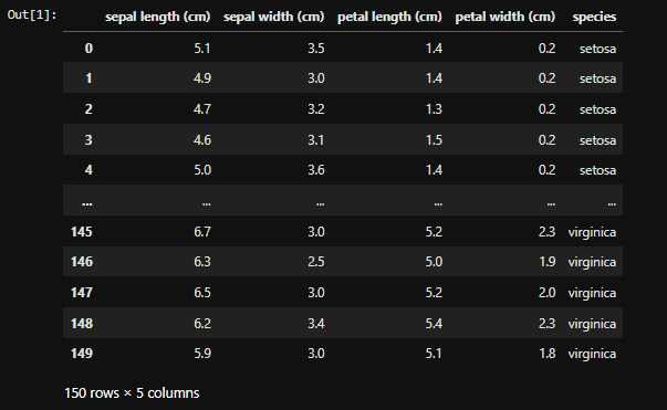
For the current project, we choose iris datasets provided by skelarn.datasets.

• Step-1: Load the datasets and create a dataframe with both the features and target variable

  
                  import pandas as pd
                  import numpy as np
                  import matplotlib.pyplot as plt
                  from sklearn import svm
                  from sklearn.datasets import load_iris
                  
                  # Load the Iris dataset
                  iris = load_iris()
                  
                  # Convert the dataset to a DataFrame
                  iris_df = pd.DataFrame(data=iris.data, columns=iris.feature_names)
                  
                  # Add the target variable (species) to the DataFrame
                  iris_df['species'] = iris.target
                  
                  # Replace target values with actual species names
                  iris_df['species'] = iris_df['species'].map({0: 'setosa', 1: 'versicolor', 2: 'virginica'})
                  
                  # Display the DataFrame
                  iris_df
              

  

• Step-2 Creating the features and target data:

  
                  # creating the Features and target data
                  # Features (input data)
                  X = iris.data
                  
                  # Target variable (output labels)
                  y = iris.target
              

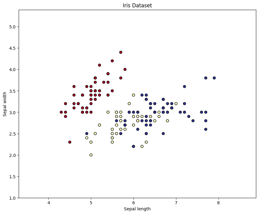
• Step-3: Now just slecting just first two columns and plotting them using scatter plot:

  
              # Create features and target data
              X = iris.data[:, :2]  # Considering only the first two features for visualization
              y = iris.target
              
              # Plotting
              x_min, x_max = X[:, 0].min() - 1, X[:, 0].max() + 1 # +/- are added for padding purpose. 
              y_min, y_max = X[:, 1].min() - 1, X[:, 1].max() + 1 # +/- are added for padding purpose. 
              
              # step size (h) for the meshgrid
              h = (x_max / x_min) / 100 # used to create a fine grid of points for visualization.
              
              # Creating a meshgrid of points
              xx, yy = np.meshgrid(np.arange(x_min, x_max, h), np.arange(y_min, y_max, h))
              # Flattening the meshgrid points into a single array
              X_plot = np.c_[xx.ravel(), yy.ravel()]
              
              # Visualize the plot
              plt.figure(figsize=(10, 8))
              
              # Plot the training points
              plt.scatter(X[:, 0], X[:, 1], c=y, cmap='RdYlBu', edgecolor='k')
              '''
              Here 
                  - c = This parameter specifies the color of each point in the scatter plot 
                  based on the values of the target variable y
              '''
              
              plt.xlim(xx.min(), xx.max())
              plt.ylim(yy.min(), yy.max())
              plt.title("Iris Dataset")
              plt.xlabel("Sepal length")
              plt.ylabel("Sepal width")
              plt.show()
              

  

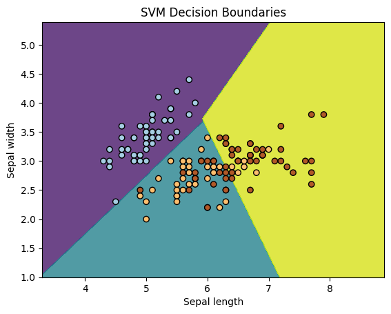
• Step-4 Using Kernels and classiying the data:

  
                  from sklearn.svm import SVC
                  from sklearn.model_selection import train_test_split
                  from sklearn.metrics import accuracy_score
                  
                  # Assuming X_train, X_test, y_train, y_test are already defined
                  
                  # Create an instance of the SVM classifier
                  svm_classifier = SVC(kernel='linear', C=1.0)
                  
                  # Train the SVM classifier
                  svm_classifier.fit(X_train, y_train)
                  
                  # Predict the labels for the test data
                  y_pred = svm_classifier.predict(X_test)
                  
                  # Evaluate the performance of the classifier
                  accuracy = accuracy_score(y_test, y_pred)
                  print("Accuracy:", accuracy)
                  # Plot decision boundaries
                  Z = svm_classifier.predict(np.c_[xx.ravel(), yy.ravel()])
                  Z = Z.reshape(xx.shape)
                  plt.contourf(xx, yy, Z, alpha=0.8)
                  
                  # Plot data points with different classes shaded or colored
                  plt.scatter(X[:, 0], X[:, 1], c=y, cmap=plt.cm.Paired, edgecolors='k')
                  plt.xlabel('Sepal length')
                  plt.ylabel('Sepal width')
                  plt.title('SVM Decision Boundaries')
                  plt.show()
              

  Accuracy: 0.9

  

  For other kernels such as Sigmoid Kernel Implementation, RBF Kernel Implementation, and Polynomial Kernel Implementation, please visit my github repo and Jupyter notebook.

On my repo, a detailed analysis of each kernel implememntation and how to choose a kernel is discussed.

References

• Confusion matrix details.
• My github Repositories on Machine learning
• Course notes on Machine learning algorithms.
• A Visual Introduction To Linear regression (Best reference for theory and visualization).
• Book on Regression model: Regression and Other Stories
• Book on Statistics: The Elements of Statistical Learning
• Naïve Bayes Classifier Algorithm, JAVAPoint.com
• https://www.colorado.edu/amath/sites/default/files/attached-files/ch12_0.pdf
• One of the best description on Linear regression.