RDD's - Resilient Distributed Datasets

Example

• Step-1: Build the SparkSession

                            # Importing Spark Session and SparkContext
                            from pyspark.sql import SparkSession
                            from pyspark import SparkContext
                            
                            # Definition of a SparkContext
                            SparkContext.getOrCreate() 
                            
                            # Definition of a SparkSession
                            spark = SparkSession \
                                .builder \
                                .master("local") \
                                .appName("Introduction to DataFrame") \
                                .getOrCreate()
                                
                            spark
                        

Here it will create a spark context and sparksession both. We will focus on SparkCOntext only here as it allows to work with RDD. So we create a SparkCOntext:

                            # Creating a shortcut to the SparkContext already created
                            sc = SparkContext.getOrCreate()
                            sc                            
                        

• Step-2Here we will load the textfile in .csv format. Next we create a rdd from the database. A rdd_row will also be created using the map, applying on each line the structure Row with the explanatory variables year, month, day and flightNum. The data file is available at Github repo.

                        # Importing Row from the pyspark.sql package
                        from pyspark.sql import Row
                        
                        # Loading the file '2008_raw.csv'
                        rdd = sc.textFile('2008_raw.csv').map(lambda line: line.split(","))
                        
                        # Creating a new rdd by selecting the explanatory variables
                        rdd_row = rdd.map(lambda line: Row(year = line[0],
                                                            month = line[1],
                                                            day = line[2],
                                                            flightNum = line[5]))
                        
                        # Creating a data frame from an rdd
                        df = spark.createDataFrame(rdd_row)
                        df.show(5) # to show the top 5 rows.
                        

• Step-3: Creating the DataFrame from a CSV using the SparkSession.

raw_df = spark.read.csv('2008.csv', header=True)

To print the schema, we can use

raw_df.printSchema()

.
• Step-4: Exploring and manipulating a DataFrame. Now we create flights1 dataframe, containing only the variables: 'year', 'month', 'day', 'flightNum', 'origin', 'dest', 'distance', 'canceled', 'cancellationCode'. and then displaying the first 20 lines:

                            # Creating a data frame containing only the explanatory variables
                            flights1 = raw_df.select('year', 'month', 'day', 'flightNum', 'origin', 'dest', 'distance', 'canceled', 'cancellationCode', 'carrierDelay')
                            
                            # Display of 20 first lines
                            flights1.show() # 'show' displays 20 lines by default
                        

Now we can also create the dataframe with a specific datatype in each column using:

                            flights = raw_df.select(raw_df.year.cast("int"),
                            raw_df.month.cast("int"),
                            raw_df.day.cast("int"),
                            raw_df.flightNum.cast("int"),
                            raw_df.origin.cast("string"),
                            raw_df.dest.cast("string"),
                            raw_df.distance.cast("int"),
                            raw_df.canceled.cast("boolean"),
                            raw_df.cancellationCode.cast("string"),
                            raw_df.carrierDelay.cast("int"))
                            
                            # Display of 20 first lines
                            flights.show()
                        

• Step-5 Some manipulation:
To count the number of flights that were delayed, you can use the following code snippet:

flights.select('flightNum').distinct().count()

Just like Pandas dataframe, we can have similar function describe to obtain a summary of the dataframe.

flights.describe().toPandas()

This will create a pandas DataFrame that contains the statistical summary for numerical columns (e.g., min, max etc).

A groupby just like python can be used to do some more analysis.

flights.groupBy('cancellationCode', 'canceled').count().show()

Summarize the variable 'cancellationCode' and 'canceled' by displaying the number of observations of each value

A filter can be used to select certain rows based on conditions.

flights.filter(flights.cancellationCode == 'C').show()

This will show the cancelled flights for the reason 'C'.

The withColumn methods allows us to create a new column.

flights.withColumn('isLongFlight', flights.distance > 1000 ).show(10)

This create a new Boolean variable isLongFlight that will be true if the flight is more than 1000 miles long and then displays first 10 line.
• Step-6: Handling missing values. Missing values appear as null in the database. There are functions such as dropna or fillna, as in module Pandas.

df.fillna( newValue, 'columnName') 

This is the syntax to handle the missing value in the column 'columnName'.

flights.fillna(0, 'carrierDelay').show(6)

To replace a value with some other value, we can use df.replace(oldValue, newValue). To replace on a specific column, we can use df.replace(oldValue, newValue, 'columnName' To replace sevral values to be replaced: df.replace([oldValue1, oldValue2], [newValue1, newValue2], 'columnName')

• Step-7: Order by operation can be used to order the dataframe according to the values of one of its variables. df.orderBy(df.age) or df.orderBy(df.age.desc()) to order the dataframe on the basis of variable age in a decreasing order.

flights.orderBy(flights.flightNum.desc()).show()

• Step-8: Spark SQL also allows you to use the SQL language. It is possible to run Pyspark using the method sql. The first step is to create a SQL view, referenced in the SQL code using the createOrReplaceTempView.

                            # Creating an SQL view
                            flights.createOrReplaceTempView("flightsView")
                            
                            # Creating a data frame containing only the variable "carrierDelay"
                            sqlDF = spark.sql("SELECT carrierDelay FROM flightsView")
                            
                            # Display of the first 10 lines
                            sqlDF.show(10)
                        

This create a SQL view of flights that will be called flightsView and then we create a DataFrame called sqlDF containing only the carrierDelay variable using a sql query. In the end we display the first line.
• Step-9: Sample and displaying tipsThe disadvantage of the method show is that it has a bad rendering when a database contains a large number of variables. It is possible to use the method toPandas to fix this problem. This method only works on a small database. To do this, the sample method returns an extract from the data, essentially taking 3 arguments:
  • withRemplacement: a Boolean to specify False if you don't want to overwrite the DataFrame
  • fraction: the fraction of data to be kept
  • seed : an integer that allows the results to be reproduced: for the same seed, a function, although random, will always give the same results
  flights.sample(False, .0001, seed = 222).toPandas() This display around ten lines of the database in an elegant way (just like pandas dataframe).

Machine learning with Pyspark Regression with PySpark

• Run the cell below to build a SparkSession for our exercise.

                            # Importing SparkSession and SparkContext
                            from pyspark.sql import SparkSession
                            from pyspark import SparkContext
                            
                            # Defining a SparkContext locally
                            sc = SparkContext.getOrCreate()
                            
                            # Building a Spark Session
                            spark = SparkSession \
                                .builder \
                                .appName("Introduction to Spark ML") \
                                .getOrCreate()
                                
                            spark
                        

• In this case, we use following dataset available at link. This dataset contains audio audio characteristics of 515345 songs released between 1922 and 2011. These songs are essentially Western commercial hits. This database contains 91 columns:
  • A variable containing the year of the song
  • 12 variables containing a 12-dimensional projection of the song's audio timbre
  • 78 variables containing audio timbre covariance information
  The objective is then to estimate the year of release of a song according to its audio characteristics. The goal is to perform a simple linear regression on the timbre information to predict the release year.
• Loading the dataset: Next we load the datafile: YearPredictionMSD.txt into a dataframe df_raw.

                            df_raw = spark.read.csv('YearPredictionMSD.txt')

                            # First display method
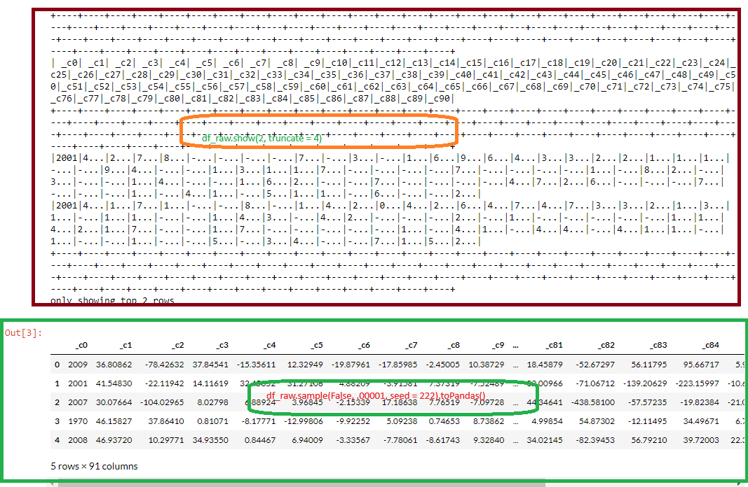
                            df_raw.show(2, truncate = 4)
                            # By modifying the values of 'truncate', this method does not allow a good visualization of the data
                            # by the number of variables
                            
                            # Second display method
                            df_raw.sample(False, .00001, seed = 222).toPandas()
                        



Displaying a database with the method show() is faster. However, the result can sometimes be incomprehensible when there are too many variables. We can then select a few variables and truncate the display to make them clean or privilege the succession of methods sample() and toPandas() taking care to choose a reasonable number of lines to display. 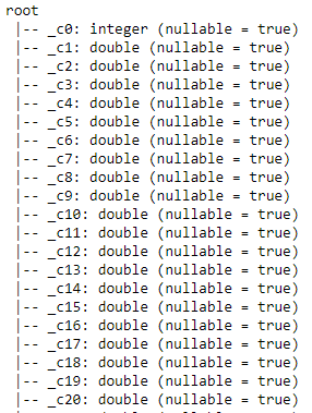It should be kept in mind that even if the sample method is relatively fast, it necessarily involves a counting of lines, a simple but slow operation in Spark. The DataSchema can be checked using df_raw.printSchema(). To change the type of each variable, it would be necessary to change its type as follows :

                                df_raw.select(df_raw._c0.cast("double"),
                                df_raw._c1.cast("double"),
                                df_raw._c2.cast("double"),
                                df_raw._c3.cast("double"),
                                ...
                                )
                            

Such a task becomes more and more tedious when the number of variables becomes large. This approach can be automated using the col function from the sub-module pyspark.sql.functions. The col function allows you to directly name a column and automate this type of approach within a loop. The next two rows then allow you to change all the columns to dual' in a new DataFrame df:

                    exprs = [col(c).cast("double") for c in df_raw.columns]
                    df = df_raw.select(*exprs)
                            

• We create dataframe df from df_raw by changing the types of columns related to the timbre to double and the year to int.

                            from pyspark.sql.functions import col

                            # Convert columns related to timbre to double and year to int
                            exprs = [col(c).cast("double") for c in df_raw.columns[1:91]]
                            df = df_raw.select(df_raw._c0.cast('int'), *exprs)
                            
                            # display of the variable schema
                            df.printSchema()
                        



To view the descriptive summary of the database df using df.describe().toPandas().
• Formatting the database in svmlib format: To be used by the Machine Learning algorithms of Spark ML, the database must be a DataFrame containing 2 columns:
  • label: containing the variable to be predicted
  • features: containing the explanatory variables.
  The DenseVector() function, from the package pyspark.ml.linalg, allows you to group several variables into one.
  Note: To be able to use the function DenseVector, we have to use the method map after transforming the DataFrame to rdd.

  
                              rdd_ml = df.rdd.map(lambda x: (x[0], 
                                  DenseVector(x[1:])))
                              # assuming that the variable to be explained is 
                              # in the first position
                              

  and then

  df_ml = spark.createDataFrame(rdd_ml, ['label', 'features'])

• Now in the present we first import DenseVector, then create rdd_ml separating the variable to be explained from the features (to be put in the form DenseVector). df_ml is created containing the database under the two variables: 'labels' and 'features'.

                            from pyspark.ml.linalg import DenseVector

                            # Creating an rdd by separating the variable to be explained from the features
                            rdd_ml = df.rdd.map(lambda x: (x[0], DenseVector(x[1:])))
                            
                            # Creation of a data frame composed of two variables: label and features
                            df_ml = spark.createDataFrame(rdd_ml, ['label', 'features'])
                            
                            # Display of the first 10 lines of the data frame
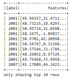
                            df_ml.show(10)
                        



• For the regression model, we create train and test datasets using train, test = df.randomSplit([.7, .3], seed= 222).

train, test = df_ml.randomSplit([.8, .2], seed= 1234)

Here this createa training DataFrame containing 70% of the data and a test one containing 30%.
• Linear Regression: Spark ML contains many Machine Learning functions. Let's start here with the most basic one: linear regression. It is present under the name LinearRegression in the module pyspark.ml.regression. This function allows you to perform a regression in a distributed way and performs calculations on the different clusters predefined in the SparkSession, regardless of their number or the size of the database. To use it, we must proceed with the two usual steps:
  • Create the function with context-specific parameters,
  • Use the fit method to apply it to the data.
  For more details on this method, we can go to following link.
  We now import the LinearRegression, create a distributed linear regression function lr to be applied to the set train. We then create linearModel, the model from lr applied to train.

                            from pyspark.ml.regression import LinearRegression

                            # Creating a linear regression function
                            lr = LinearRegression(labelCol='label', featuresCol= 'features')
                            
                            # Fitting of training data "train".
                            linearModel = lr.fit(train)
                        

• Now that the learning model is built, it is possible to predict labels on the test data. To do this, the Spark ML models have a transform() method to make predictions using only the test set as an argument.

                            predicted = linearModel.transform(test)

                            # Printing prediction
                            predicted.show()
                        

• Model evaluation: In order to evaluate the quality of the model, it is possible to search for information within the summary attribute of our model, which can be done through function linearModel.summary.

                            print("RMSE:", linearModel.summary.rootMeanSquaredError)

                            print("R2:  ", linearModel.summary.r2)
                        

Here we display the RMSE and R² values.

                            RMSE: 9.548411838648486
                            
                            R2:   0.2363424607632092
                        

• Coefficients: We can calculate the Coefficients using:

                            from pprint import pprint
                            pprint(linearModel.coefficients)

which shows:

DenseVector([0.876, -0.0562, -0.0439, 0.0036, -0.0149, -0.2193, -0.0071, -0.0997, -0.0705, 0.0263, -0.1676, -0.0002, 0.0466, 0.0004, -0.0004, 0.0006, 0.0005, 0.0014, 0.002, 0.0021, 0.0007, -0.0001, 0.0074, 0.0029, -0.0036, 0.0001, 0.0016, 0.0005, 0.001, -0.0003, -0.0013, -0.0015, -0.0054, 0.0026, 0.0017, -0.0052, -0.0003, 0.0007, 0.0014, -0.0016, -0.0019, -0.0008, -0.0014, -0.0024, -0.0033, 0.0067, 0.0005, -0.0021, 0.0003, 0.0019, 0.0002, -0.0016, 0.0019, 0.0004, -0.0, 0.0002, -0.002, 0.0019, -0.0013, 0.0002, -0.0031, -0.002, -0.0075, 0.0012, -0.0021, 0.0006, -0.0001, -0.0004, -0.0043, -0.0052, -0.0011, 0.0002, 0.0007, 0.004, 0.0028, 0.0156, 0.0002, -0.0044, -0.0002, -0.0002, -0.0002, -0.0005, 0.0013, 0.0011, 0.0257, 0.0002, 0.0011, -0.0309, -0.0014, -0.0014])
                        

References

1. Official Documentation
2. Databricks Learning Academy
3. Spark by Examples
4. Datacamp tutorial.
5. For databricks, you can look at tutorial videos on youtube at youtube video by Bryan Cafferky, writer of the book "Master Azure Databricks". A great playlist for someone who just want to learn about the big data analytics at Databricks Azure cloud platform.
6. See the video for pyspark basics by Krish Naik. Great video for starter.
7. Great youtube on Apache spark one premise working.