Random Variables

A random variable is a numerical description of the outcome of a statistical experiment. A random variable that may assume only a finite number or an infinite sequence of values is said to be discrete; one that may assume any value in some interval on the real number line is said to be continuous

A random variable can be classified as:

Discrete random variable:
- Takes on a countable number of distinct values.
- Examples include the number of heads in multiple coin tosses or the count of occurrences in a specific time period.
- Discrete random variable are described using "Probability mass Function (PMF)" and "Cumulative Distribution Function (CDF)".
- PMF is the probability that a random variable X takes a specific value k; for example. the number of fraudulent transactions at an e-commerce platform is 10, written as $P(X=10)$. On the other hand, CDF is the probability that a random variable X, takes a value less than or equal to 10 which is written as $P(X\leq 10)$.
Continuous random variable
- A random variable $X$ which can take a value from an infintie set of values is called a continuous random variable.
- Examples include measurements like height, weight, or time intervals.
- Continuous random variables are described using "Probability Desnity Function (PDF)", and "Cumulative Distribution Fnction (CDF)". PDF is the probability that a continuous random variable $X$ takes value in a small neighbourhood of "$x$" and is given by: $$f(x) = \text{Lim}_{\delta x \rightarrow 0} P[x\leq X \leq x+\delta x].$$ The CDF of a continuous random varibale is the probability that the random variable $X$ takes value less than or equal to a value "$a$". Mathematically: $$F(a) = \int_{-\infty }^\infty f(x) dx.$$

Probability distributions

A probability distribution is a function that describes the likelihood of each possible outcome in a random experiment. Variables that follow a probability distribution are called random variables. In other words, it is a mathematical function that assigns probabilities to all possible outcomes of a random variable. There are two types of probability distributions:

Discrete distributions,
Continuous distributions.

Next we will discuss each one of them, one by one.

Discrete distributions

A discrete probability distribution assigns probabilities to a finite or countably infinite number of possible outcomes. There are several types of discrete probability distributions, including:

1. Bernoulli distribution

The Bernoulli distribution is a simple probability distribution that describes the probability of success or failure in a single trial of a binary experiment. The Bernoulli distribution has two possible outcomes: success (with probability $p$) or failure (with probability $1-p$). The formula for the Bernoulli distribution is:

$$P(X=x) = p^x \times (1-p)^{(1-x)}$$ where $X$ is the random variable, $x$ is the outcome (either $0$ or $1$), and $p$ is the probability of success.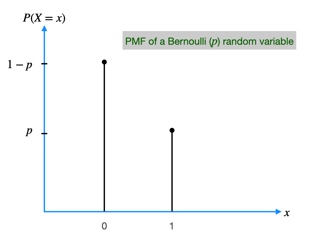

Bernoulli Distribution
Random Variable	X ∈ {0, 1} P(X = 1) = p, P(X = 0) = 1 − p
Mean (Expected Value)	μ = E[X] = p
Variance	Var(X) = p(1 − p)
Standard Deviation	σ = √[p(1 − p)]
Moment Coefficient of Skewness	γ₁ = (1 − 2p) / √[p(1 − p)]
Moment Coefficient of Kurtosis	γ₂ = (1 − 6p(1 − p)) / (p(1 − p))

2. Binomial distribution

The binomial distribution describes the probability of getting a certain number of successes in a fixed number of independent trials of a binary experiment. The binomial distribution has two parameters: $n$, the number of trials, and $p$, the probability of success in each trial. The formula for the binomial distribution is: $$P(X=x) = ^nC_x ~ p^x ~ (1-p)^{(n-x)}$$ where $X$ is the random variable representing the number of successes, $x$ is the number of successes, $n$ is the number of trials, $p$ is the probability of success, and $^nC_x = \frac{n!}{x! (n-x)!}$ is the binomial coefficient, which represents the number of ways to choose $x$ objects from a set of n objects.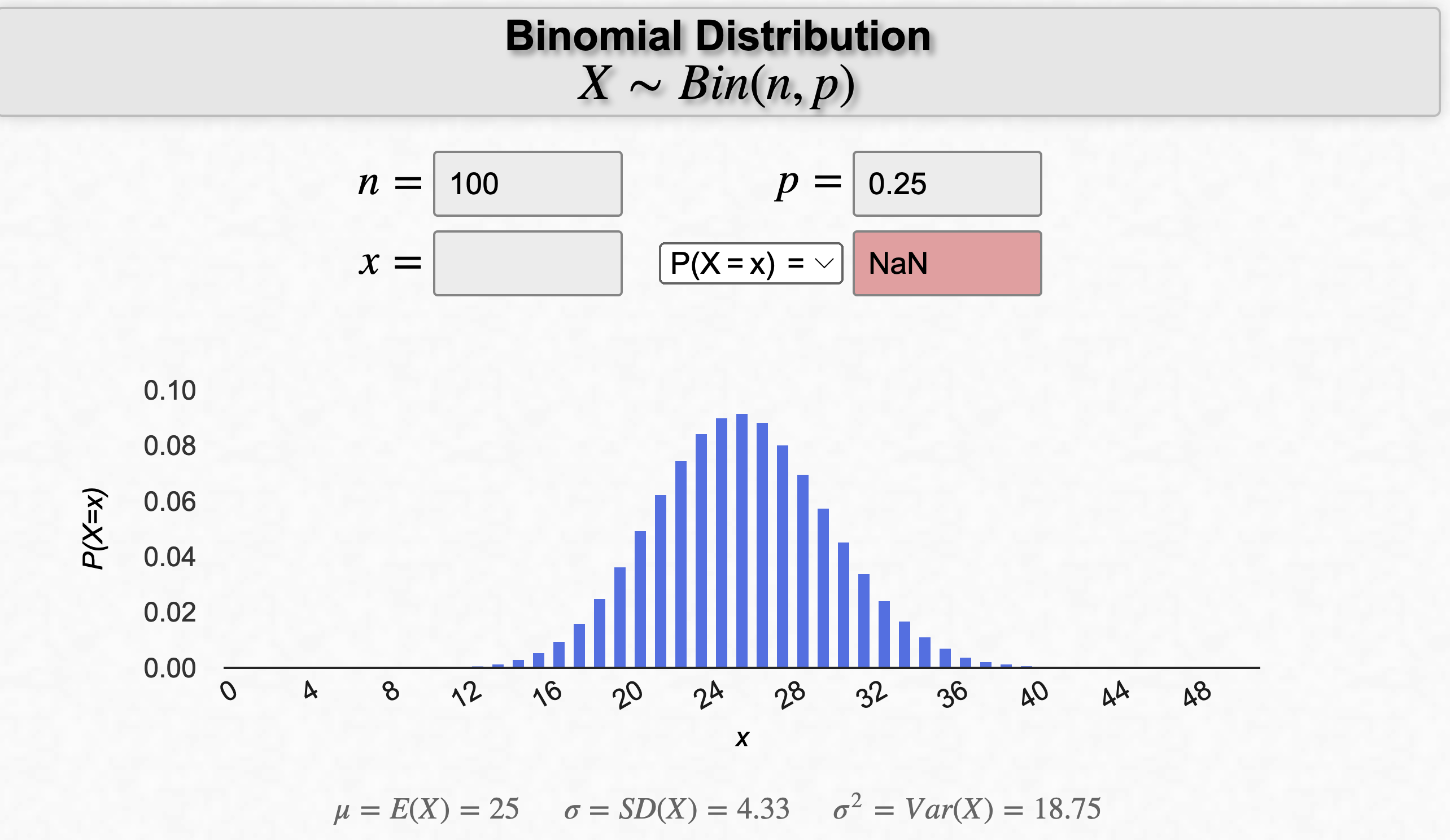

Statistic	Formula
Mean	$$\mu = np$$
Variance	$$\sigma^2 = np(1 - p)$$
Standard Deviation	$$\sigma = \sqrt{np(1 - p)}$$
Moment Coefficient of Skewness	$$\alpha_3 = \frac{1 - 2p}{\sqrt{np(1 - p)}}$$
Moment Coefficient of Kurtosis	$$\alpha_4 = 3 + \frac{1 - 6p(1 - p)}{np(1 - p)}$$

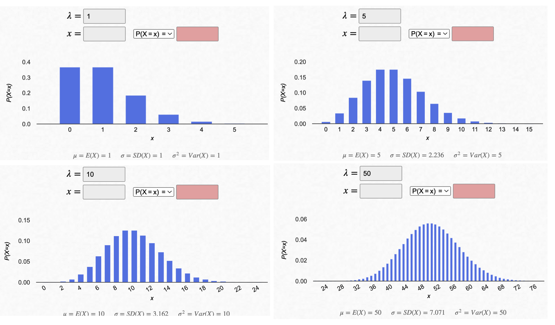
3. Poisson distribution

The Poisson distribution is used to describe the probability of a certain number of events occurring in a fixed time interval when the events occur independently and at a constant rate. The Poisson distribution has one parameter: $\lambda$, which represents the expected number of events in the time interval. The formula for the Poisson distribution is:

$$P(X=x) = e^{-λ} \frac{λ^x}{x!}$$

where $X$ is the random variable representing the number of events, $x$ is the number of events, $e$ is the mathematical constant, $\lambda$ is the expected number of events, and $x!$ is the factorial function.

Statistic	Formula
Mean	$$\mu = \lambda$$
Variance	$$\sigma^2 = \lambda$$
Standard Deviation	$$\sigma = \sqrt{\lambda}$$
Moment Coefficient of Skewness	$$\alpha_3 = \frac{1}{\sqrt{\lambda}}$$
Moment Coefficient of Kurtosis	$$\alpha_4 = 3 + \frac{1}{\lambda}$$

Continuous distributions

Continuous probability distributions are used to model continuous random variables, which can take on any value in a given range. Unlike discrete random variables, which take on only a finite or countably infinite set of possible values, continuous random variables can take on an uncountably infinite set of possible values. There are several common continuous probability distributions, including:

1. Normal distribution

also known as the Gaussian distribution, this is a bell-shaped distribution that is symmetric around the mean. It is commonly used to model measurements that are expected to be normally distributed, such as heights or weights of individuals in a population. The probability density function (PDF) of the normal distribution is:

$$f(x; \mu, \sigma) = \frac{1}{\sigma \sqrt{2\pi}} \text{Exp}\left(-\frac{(x-\mu)^2}{2\sigma^2}\right)$$ where $x$ is the random variable, $\mu$ is the mean, $\sigma$ is the standard deviation.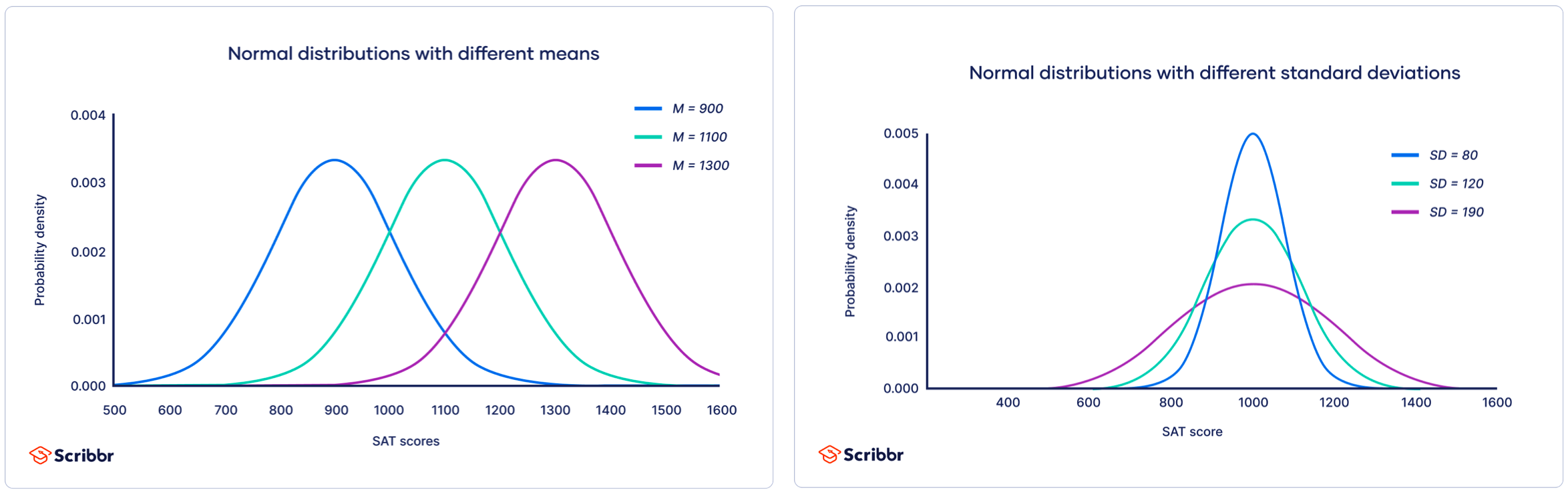

The Empirical Rule, also known as the 68-95-99.7 Rule, is a rule of thumb for the normal distribution. It states that:

Approximately 68% of the data falls within one standard deviation of the mean.
Approximately 95% of the data falls within two standard deviations of the mean.
Approximately 99.7% of the data falls within three standard deviations of the mean.

This means that if a distribution is approximately normal, we can use these percentages to estimate the proportion of data that falls within a certain range of values.

It's important to note that the Empirical Rule is only an approximation and may not hold for all normal distributions. It is also not applicable to non-normal distributions.

Statistic	Formula
Mean	$$\mu$$
Variance	$$\sigma^2$$
Standard Deviation	$$\sigma$$
Moment Coefficient of Skewness	$$\alpha_3 = 0$$
Moment Coefficient of Kurtosis	$$\alpha_4 = 3$$
Mean Deviation	$$\sigma \sqrt{\frac{2}{\pi}} \approx 0.7979\,\sigma$$

Generating distribution function in python


                            # Generate Normal Distribution
                            normal_dist = np.random.randn(10000)
                            normal_df = pd.DataFrame({'value' : normal_dist})
                            # Create a Pandas Series for easy sample function
                            normal_dist = pd.Series(normal_dist)
                            
                            normal_dist2 = np.random.randn(10000)
                            normal_df2 = pd.DataFrame({'value' : normal_dist2})
                            # Create a Pandas Series for easy sample function
                            normal_dist2 = pd.Series(normal_dist)
                            
                            normal_df_total = pd.DataFrame({'value1' : normal_dist, 
                                                            'value2' : normal_dist2}) 
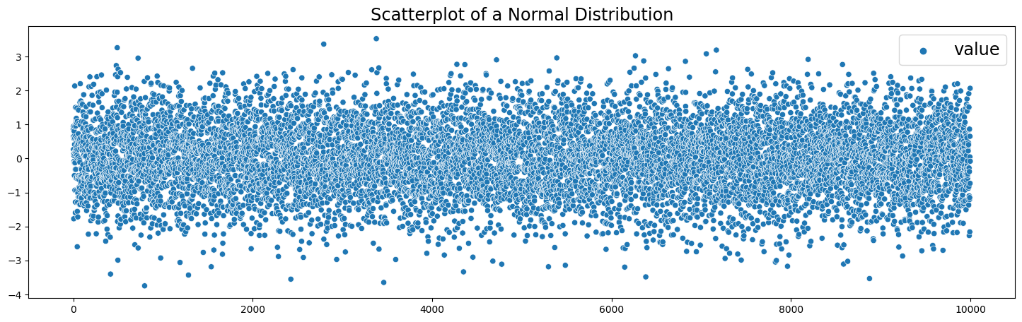
                                                            # Scatterplot
                                                            plt.figure(figsize=(18,5))
                                                            sns.scatterplot(data=normal_df)
                                                            plt.legend(fontsize='xx-large')
                                                            plt.title('Scatterplot of a Normal Distribution', fontsize='xx-large')


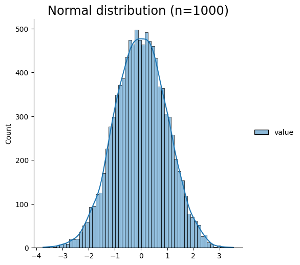
                            # Normal Distribution as a Bell Curve
                            plt.figure(figsize=(18,5))
                            sns.displot(normal_df, kde=True)
                            plt.title('Normal distribution (n=1000)', fontsize='xx-large')
                            plt.show()


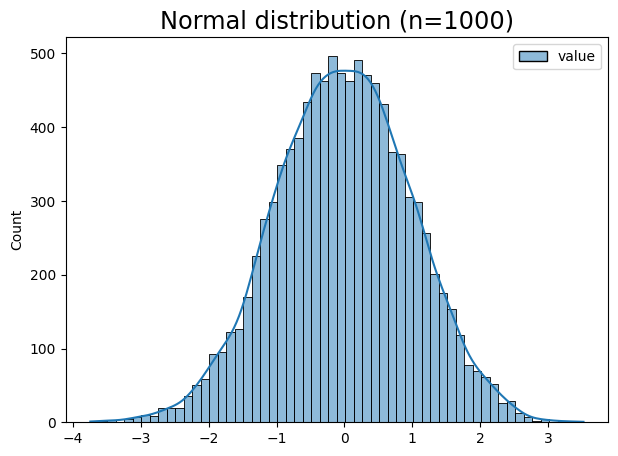
                            plt.figure(figsize=(7,5))
                            sns.histplot(normal_df, kde=True)
                            plt.title('Normal distribution (n=1000)', fontsize='xx-large')
                            plt.show()

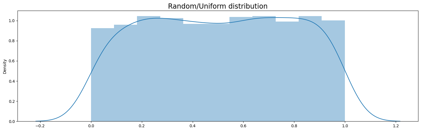
2. Uniform distribution

this is a distribution in which all values in a given range are equally likely to occur. The PDF of the uniform distribution is: $$f(x)= \begin{cases} \frac{1}{b-a}, & a \leq x \leq b \\ 0, & \text{otherwise} \end{cases}$$ where $x$ is the random variable, $a$ is the lower bound of the range, and $b$ is the upper bound of the range.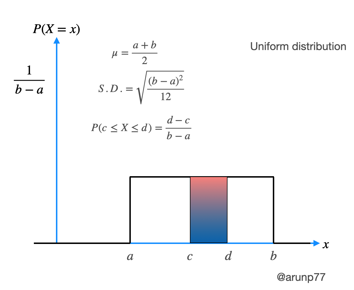

3. Exponential distribution

this is a distribution that is commonly used to model the time between events that occur at a constant rate. The PDF of the exponential distribution is:

$$ f(x; \lambda) = \begin{cases} \lambda e^{-\lambda x}, & x \geq 0 \\ 0, & x < 0 \end{cases} $$ where $x$ is the random variable, and $\lambda$ is the rate parameter.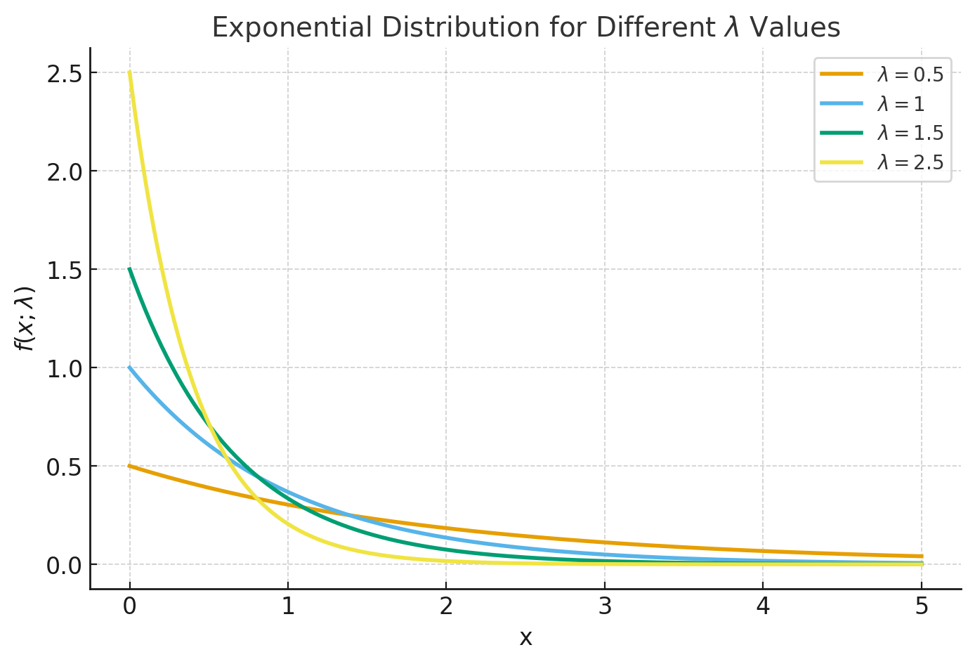

In this example we generate random floating numbers between 0 and 1.

The PDF of a Uniform Distribution:

$$ f(x)= \begin{cases} \frac{1}{b-a}, & a \leq x \leq b \\ 0, & \text{otherwise} \end{cases} $$

CDF:

$$ CDF = \begin{cases} 0, & x < a \\ \frac{x-a}{b-a} & a \leq x \leq b \\ 1 & for x\geq b \end{cases} $$


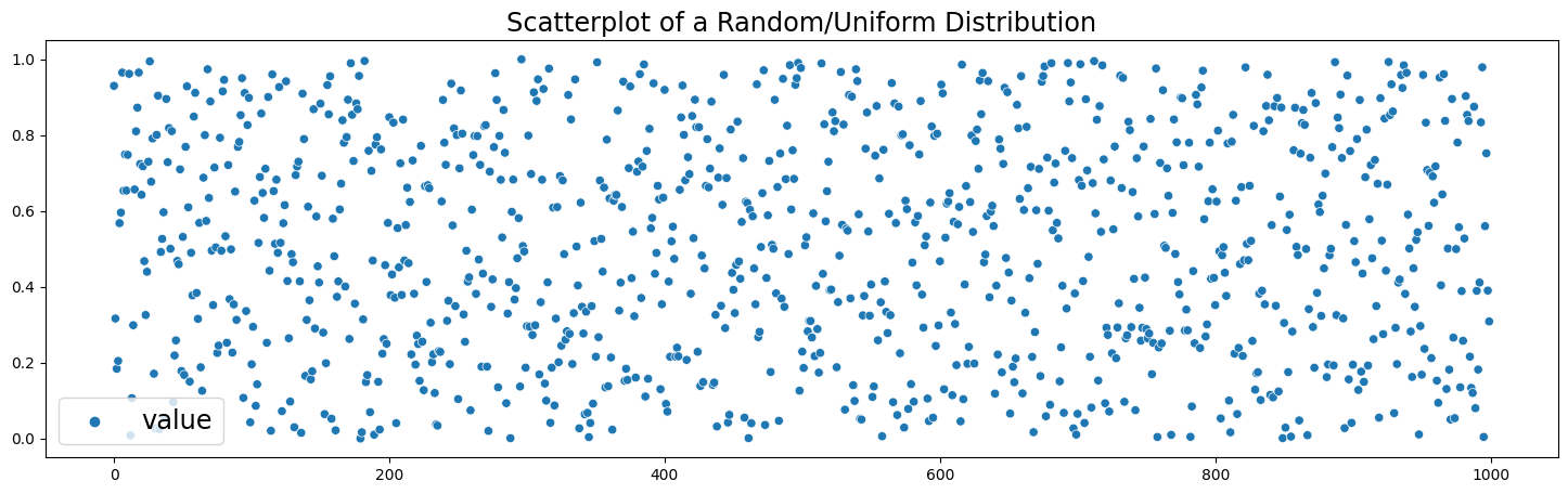
                            # Uniform distribution (between 0 and 1)
                            uniform_dist = np.random.random(1000)
                            uniform_df = pd.DataFrame({'value' : uniform_dist})
                            uniform_dist = pd.Series(uniform_dist) 
                            plt.figure(figsize=(18,5))
                            sns.scatterplot(data=uniform_df)
                            plt.legend(fontsize='xx-large')
                            plt.title('Scatterplot of a Random/Uniform Distribution', fontsize='xx-large')


                            plt.figure(figsize=(18,5))
                            sns.distplot(uniform_df)
                            plt.title('Random/Uniform distribution', fontsize='xx-large')

3. Gamma distribution

this is a distribution that is used to model the sum of several exponentially distributed random variables. The PDF of the gamma distribution is: $$f(x; k, \theta) = \frac{x^{k-1} e^{-x/\theta}}{\theta^k \Gamma(k)}$$ where $x$ is the random variable, $k$ is the shape parameter, $\theta$ is the scale parameter, and $\Gamma(k)$ is the gamma function.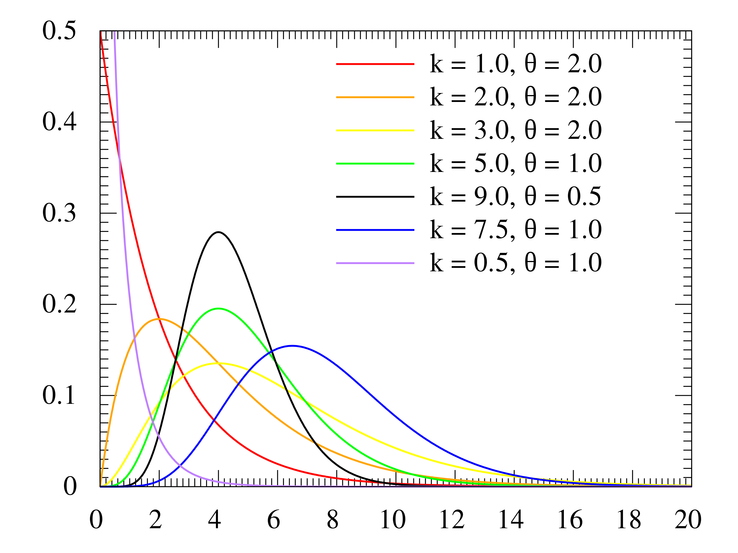

The probability distribution is an essential concept in probability theory and is used to calculate the expected values, variances, and other statistical properties of random variables. Understanding probability distributions is important in fields such as statistics, physics, engineering, finance, and many others where randomness plays a role.

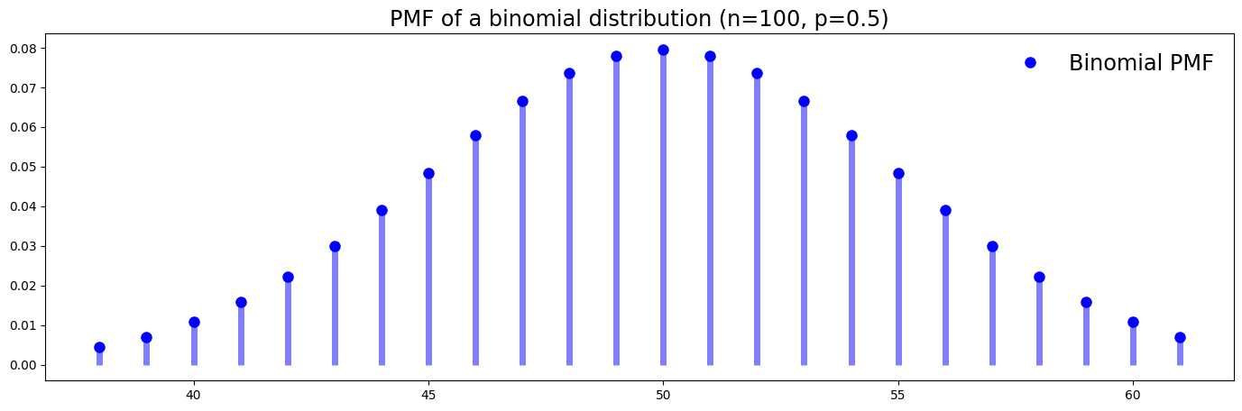
PMF (Probability Mass Function)

Here we visualize a PMF of a binomial distribution. You can see that the possible values are all integers. For example, no values are between 50 and 51. The PMF of a binomial distribution in function form:

$$P(X=x)= p^x\left(\frac{N}{x}\right)(1-p)^{N-x}$$


                            # PMF Visualization
                            n = 100
                            p = 0.5
                            
                            fig, ax = plt.subplots(1, 1, figsize=(17,5))
                            x = np.arange(binom.ppf(0.01, n, p), binom.ppf(0.99, n, p))
                            ax.plot(x, binom.pmf(x, n, p), 'bo', ms=8, label='Binomial PMF')
                            ax.vlines(x, 0, binom.pmf(x, n, p), colors='b', lw=5, alpha=0.5)
                            rv = binom(n, p)
                            #ax.vlines(x, 0, rv.pmf(x), colors='k', linestyles='-', lw=1, label='frozen PMF')
                            ax.legend(loc='best', frameon=False, fontsize='xx-large')
                            plt.title('PMF of a binomial distribution (n=100, p=0.5)', fontsize='xx-large')
                            plt.show()

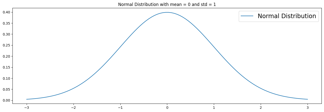
PDF (Probability Density Functions)

The PDF is the same as a PMF, but continuous. It can be said that the distribution has an infinite number of possible values. Here we visualize a simple normal distribution with a mean of 0 and standard deviation of 1.


                            # Plot normal distribution
                            mu = 0
                            variance = 1
                            sigma = sqrt(variance)
                            x = np.linspace(mu - 3*sigma, mu + 3*sigma, 100)
                            plt.figure(figsize=(16,5))
                            plt.plot(x, stats.norm.pdf(x, mu, sigma), label='Normal Distribution')
                            plt.title('Normal Distribution with mean = 0 and std = 1')
                            plt.legend(fontsize='xx-large')
                            plt.show()

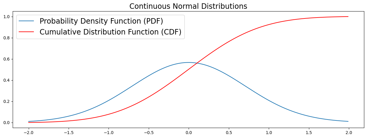
CDF (Cumulative Distribution Function)

The CDF maps the probability that a random variable $X$ will take a value of less than or equal to a value $x$ ($P(X ≤ x)$). CDF's can be discrete or continuous. In this section we visualize the continuous case. You can see in the plot that the CDF accumulates all probabilities and is therefore bounded between $0 \leq x \leq 1$.


                            # Data
                            X  = np.arange(-2, 2, 0.01)
                            Y  = exp(-X ** 2)
                            
                            # Normalize data
                            Y = Y / (0.01 * Y).sum()
                            
                            # Plot the PDF and CDF
                            plt.figure(figsize=(15,5))
                            plt.title('Continuous Normal Distributions', fontsize='xx-large')
                            plot(X, Y, label='Probability Density Function (PDF)')
                            plot(X, np.cumsum(Y * 0.01), 'r', label='Cumulative Distribution Function (CDF)')
                            plt.legend(fontsize='xx-large')
                            plt.show()

Distribution Functions – Python Examples

Reference:

Visit the "Learn about PostgreSQL"
Visit the "DBMS Tutorials page"
Visit my "Github repository on SQL" to learn about basics and some example projects.
Visit my "Github repository" to learn about databases.