
Unraveling the Mysteries of the Early Universe: Exploring Dark Matter Ionization with LOFAR Data
Introduction
The early universe holds many secrets, and unraveling its mysteries requires cutting-edge tools and techniques. In recent years, radio interferometry has emerged as a powerful tool for studying the universe's infancy. In this article, we delve into groundbreaking research conducted using data from the Low Frequency Array (LOFAR) to investigate the dark matter ionization history during the reionization-recombination epoch.Understanding LOFAR Data:
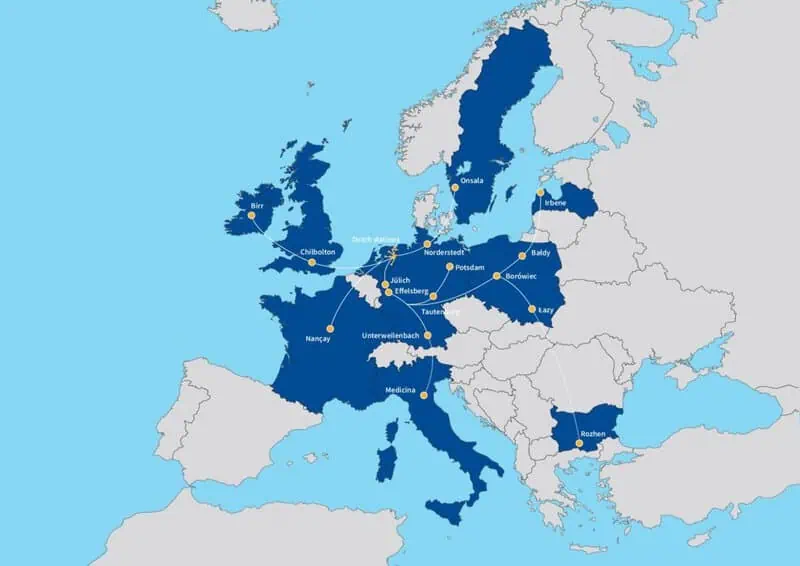
LOFAR, the Low Frequency Array, is a state-of-the-art radio telescope network spanning multiple countries in Europe. Designed to observe the universe in the low-frequency radio range, LOFAR produces vast datasets capturing radio emissions from celestial sources. Among these datasets, raw visibilities play a crucial role. Raw visibilities are the correlated signals between pairs of antennas, capturing the interference pattern of radio waves from the early universe.Research Objective:
The primary objective of our research is to trace the ionization history of dark matter during the reionization-recombination epoch using LOFAR data. This epoch marks a crucial period in the universe's evolution when the first stars and galaxies formed, and neutral hydrogen was gradually ionized by the intense radiation from these sources. By studying the ionization patterns, we aim to shed light on the role of dark matter in this cosmic transition.Data Collection and Conversion
Our research begins with the collection of raw visibilities from the LOFAR telescope network. These visibilities, representing correlated signals between antenna pairs, are then processed and calibrated to remove instrumental and atmospheric effects. Calibration is followed by imaging, where Fourier transforms are applied to convert visibilities into detailed images of the radio sky. Through this process, we obtain image cubes and spectral line data, which form the basis of our analysis.Analysis Methodology
The heart of our research lies in the analysis of LOFAR data to extract insights into the ionization history of dark matter. We focus on several key aspects:- Mapping Neutral Hydrogen Distribution: Using 3D data cubes generated from LOFAR data, we map the distribution of neutral hydrogen over different redshifts. By studying the spatial and temporal variations in hydrogen density, we gain valuable insights into the ionization process.
- Analyzing the 21 cm Hydrogen Line: The 21 cm hydrogen line is a powerful tool for probing the universe's ionization state. By analyzing spectral line data from LOFAR, we study deviations in the 21 cm signal to infer the presence and influence of dark matter.
- Removing Foreground Contamination: To isolate the cosmic signal from the epoch of reionization, we utilize source catalogs generated from LOFAR data. By identifying and filtering out foreground sources, such as nearby galaxies and quasars, we ensure the accuracy of our analysis.
Scientific Impact and Future Directions
Our research holds significant implications for our understanding of the early universe and the role of dark matter in cosmic evolution. By leveraging LOFAR data, we aim to contribute to the growing body of knowledge on the reionization-recombination epoch and its implications for cosmology and astrophysics. Looking ahead, we envision further advancements in data analysis techniques and the continued exploration of the radio sky with next-generation instruments.Conclusion
In conclusion, our research represents a pioneering effort to probe the dark matter ionization history during the reionization-recombination epoch using LOFAR data. By combining cutting-edge observational data with sophisticated analysis techniques, we strive to unlock the secrets of the early universe and deepen our understanding of cosmic evolution.Data collection, conversion, and usage
Let's first understand the data collection, conversion and it's usage step by step.- Data Collection: Raw Data: Signals from the early universe travel as electromagnetic waves. These waves include the 21 cm hydrogen line, which is particularly important for studying the early universe. Radio telescopes detect these electromagnetic waves. The signals are captured by multiple antennas arranged in an array (e.g., LOFAR). A central system correlates the signals from each pair of antennas, producing complex numbers representing the amplitude and phase difference (visibility). Here amplitude indicates the strength of the correlated signal and the phase represents the phase difference due to the path length difference between the antennas. Visibilities are not the direct observations of electromagnetic waves but rather the result of processing the signals captured by pairs of antennas. When two antennas receive the same signal from a celestial source, the difference in the arrival time of the signal at each antenna (due to their spatial separation) creates an interference pattern. The correlator (a central processing unit) combines these signals to produce a complex number (visibility), which encodes both amplitude and phase information.
- Type: Raw visibilities
- Source: LOFAR (Low Frequency Array) telescope network
- Content: Correlated signals between pairs of antenna stations, represented as complex numbers.
- Purpose: To capture radio emissions from the early universe, particularly the 21 cm hydrogen line.
- Data Conversion:
- Pre-processing:
- RFI Mitigation: Remove radio frequency interference from human-made sources.
- Flagging: Identify and exclude bad or corrupted data.
- Calibration:
- Instrumental Calibration: Correct for antenna gains, clock drifts, and other instrumental effects.
- Ionospheric Calibration: Correct for distortions caused by the Earth's ionosphere.
- Output: Calibrated visibilities that accurately represent the sky's radio emissions.
- Imaging:
- Fourier Transform: Convert calibrated visibilities into image cubes (2D sky coordinates + 1 frequency axis).
- Deconvolution: Remove artifacts and enhance image quality.
- Output: Image cubes and spectral line data.
- Pre-processing:
- Data Usage for Research: Analyzing Image Cubes
- Analyzing Image Cubes:
- Neutral Hydrogen Mapping: Use 3D data cubes to map the distribution of neutral hydrogen over different redshifts (distances/times).
- Frequency Analysis: Focus on the 21 cm hydrogen line to study the ionization state of hydrogen in the early universe.
- Spectral Line Data:
- 21 cm Emission: Detect and analyze the 21 cm signal, which provides insights into the density and temperature of neutral hydrogen.
- Dark Matter Interactions: Infer the impact of dark matter on hydrogen ionization by analyzing deviations in the expected 21 cm signal.
- Source Catalogs:
- Foreground Removal: Identify and filter out foreground sources (e.g., nearby galaxies, quasars) to isolate the cosmic signal.
- Cross-Referencing: Use catalogs to ensure accurate identification and removal of non-relevant sources
- Polarization Data:
- Magnetic Field Effects: Understand and correct for the influence of cosmic magnetic fields on the observed signal.
- Foreground Correction:Use polarization data to further refine the cosmic signal by removing polarized foreground contamination.
- Analyzing Image Cubes:
Raw Visibilities
When we talk about visibilities in the context of radio interferometry, we are dealing with complex numbers that encapsulate both the amplitude and phase of the correlated signal between pairs of antennas (baselines). Visibility as a complex number is defined as: $$V(u,v) = A(u,v) e^{i\phi(u,v)}$$ where- \(A(u,v)\) is the amplitude of the visibility, indicating the strength of the correlated signal.
- \(\phi(u,v)\) is the phase of the visibility, representing the phase difference between the signals received by the two antennas.
- \((u,v)\) are the coordinates of the baseline in the uv-plane, which corresponds to the spatial frequency, measured in wavelengths.
Phase Difference and Path Length Difference: The phase difference \(\phi\) is related to the path length difference \(\Delta L\) between the signals arriving at the two antennas. This path length difference occurs because the antennas are spatially separated, and the wavefront from a distant source reaches each antenna at slightly different times. The phase difference is given by:
$$\phi = \frac{2\pi \Delta L}{\lambda}$$ where,- \(\Delta L\) is the path length difference between the two antennas.
- \(\lambda\) is the wavelength of the observed electromagnetic wave.
Visibility Formula Incorporating Phase Difference Given the path length difference, the visibility can be expressed in terms of its real and imaginary components:
$$V(u,v) = A(u,v) \cdot \left(\cos \phi + i \sin \phi\right)$$ So in this form, the visibility is composed of a real and a c=imaginary part.Deriving Brightness Distribution
Raw visibilities are the correlated signals between pairs of antennas (also called baselines) in a radio interferometer array. These measurements capture the interference pattern of radio waves from celestial sources. The visibility \(V(u,v)\) for a given basline (pair of antennas) is essentially the Fourier transform of the sky brightness distribution \(I(l,m)\). i.e. to convert visibilities into a sky brightness distribution \(I(l,m)\), we use the inverse Fourier transform: $$V(u,v) = \int\int I(l,m) ~\text{exp}[-2\pi i (ul+vm)] dl dm$$ where:- \(I(l,m)\)is the sky brightness distribution as a function of direction cosines \(l\) and \(m\), which are projections of the source position on the sky.
- \((l,m)\)are direction cosines relative to the center of the field of view.
Key Components:
- Baseline Coordinates \((u,v)\): Each baseline (pair of antennas) provides a sample point in the uv-plane.
- Sky brightness Distribution \(I(l,m)\): Represents the intensity of radio emission from different directions on the sky.
- Exponential Term \((\text{exp}[-2\pi i (ul+vm)])\):The phase term that captures the delay between signals received by the antennas due to their spatial separation.
Example: Consider two antennas separated by a distance \(d\) in the east-west direction. The baseline \(u\) is given by:
$$u = \frac{d}{\lambda}$$ where \(\lambda\) is the wavelength of the observed radio waves. For a point source at an angle \(\theta\) from the zenith, the visibility \(V(u,v)\) can be simplified as: $$V(u,v) = I_0 ~\text{exp}[-2\pi i \frac{d}{\lambda}~\sin \theta]$$ here, \(I_0\) is the intrinsic brightness of the point source.Brightness temperature: The sky brightness distribution \(I(l,m)\) from the images is used to calculate the brightness temeprature \(T_b\).
$$T_b = \frac{c^2 I_\nu}{2 k_B \nu^2}$$ where \(I_\nu\) is the specific intensity (brightness), \(c\) is the speed of light, \(k_B\) is the Boltzmann constant, and \(\nu\) is the frequency of observation.By measuring the visibilities of incoming radio signals and converting them into the sky brightness distribution, we can calculate the brightness temperature. This brightness temperature provides a wealth of information about the early universe, including the temperatures of baryons and dark matter. Through careful analysis of these temperatures, we can gain insights into the ionization history during the reionization-recombination epoch, thereby enhancing our understanding of cosmic evolution and the role of dark matter.
Common data file structure:
A common data file from LOFAR typically contains a variety of information necessary for radio interferometric analysis. These files often come in standardized formats, such as Measurement Sets (MS), which are designed to store the complex and voluminous data produced by radio interferometers. Here is a breakdown of the key information contained in a typical LOFAR data file:- Visibility Data:
- Amplitude and Phase: Complex numbers representing the amplitude and phase of the correlated signals between pairs of antennas.
- Time Stamps: The exact times when each visibility measurement was taken.
- Baseline Information: Data on the specific pairs of antennas (baselines) involved in each measurement.
- Antenna Information:
- Antenna Positions: The precise geographical locations of the antennas in the array, usually given in Cartesian coordinates (x, y, z).
- Antenna Identifiers: Unique IDs or names for each antenna in the array.
- Frequency Information:
- Frequency Channels: The specific frequencies or channels at which the observations were made.
- Bandwidth: The width of each frequency channel.
- Observation Metadata:
- Source Information: Details about the celestial source(s) being observed, including coordinates (right ascension and declination).
- Observation Time: The start and end times of the observation period.
- Pointing Direction: The direction in which the antennas were pointed during the observations.
- Calibration Information:
- Calibration Tables: Data used to correct for instrumental and atmospheric effects, including information on gain, phase, and bandpass calibration.
- Flagging Information: Data indicating which visibilities have been flagged (excluded) due to issues such as radio frequency interference (RFI) or other problems.
- Auxiliary Data:
- Weather Data: Environmental information that might affect the observations, such as temperature, humidity, and atmospheric pressure.
- System Logs: Logs and diagnostics from the telescope system during the observation period.
Example Structure of a LOFAR Measurement Set (MS) File: A Measurement Set file typically includes multiple tables, each storing different aspects of the observation data. Commonly such files are given as HDF5 file. HDF5 (Hierarchical Data Format version 5) is a file format and set of tools for managing complex data. It's used to store and organize large amounts of data, such as those produced by scientific computations, which makes it suitable for storing LOFAR data. The data would be organized hierarchically in groups and datasets. Each group represents a logical section of the data, and datasets store the actual data arrays. Below is an example structure for the LOFAR data file. Here is an example of the structure:
- MAIN Table: Following are the columns
- DATA: The complex visibility data (amplitude and phase).
- TIME: The time of the measurement.
- ANTENNA1, ANTENNA2: Identifiers for the pair of antennas.
- UVW: Baseline coordinates in the uvw-space.
- FLAG: Flagging status for each visibility.
- ANTENNA Table:
- POSITION: The x, y, z coordinates of each antenna.
- NAME: The name or ID of each antenna.
- SPECTRAL_WINDOW Table:Following are the columns
- NUM_CHAN: The number of frequency channels.
- REF_FREQUENCY: The reference frequency of the observation.
- CHAN_WIDTH: The width of each frequency channel.
- FIELD Table:
Following are the columns
- NAME: The name of the observed field.
- PHASE_DIR: The pointing direction of the array (right ascension and declination).
- OBSERVATION Table: Following are the columns
- START_TIME: The start time of the observation.
- END_TIME: The end time of the observation.
- OBSERVER: The name of the observer or observing team.
- CALIBRATION Tables: Following are the columns
- Separate tables for gain, bandpass, delay, and other calibration parameters.
                / (root)
                |
                |-- /VisibilityData
                |   |-- /Amplitude
                |   |-- /Phase
                |   |-- /TimeStamps
                |   |-- /BaselineInformation
                |
                |-- /AntennaInformation
                |   |-- /AntennaPositions
                |   |-- /AntennaIdentifiers
                |
                |-- /FrequencyInformation
                |   |-- /FrequencyChannels
                |   |-- /Bandwidth
                |
                |-- /ObservationMetadata
                |   |-- /SourceInformation
                |   |-- /ObservationTime
                |   |-- /PointingDirection
                |
                |-- /CalibrationInformation
                |   |-- /CalibrationTables
                |   |-- /FlaggingInformation
                |
                |-- /AuxiliaryData
                    |-- /WeatherData
                    |-- /SystemLogs
- /VisibilityData
- /Amplitude: Dataset storing the amplitudes of the visibilities.
- /Phase: Dataset storing the phases of the visibilities.
- /TimeStamps: Dataset storing the exact times when each visibility measurement was taken.
- /BaselineInformation:Dataset storing information on the specific pairs of antennas involved in each measurement.
- /AntennaInformation
- /AntennaPositions: Dataset storing the precise geographical locations of the antennas in the array (Cartesian coordinates: x, y, z).
- /AntennaIdentifiers: Dataset storing unique IDs or names for each antenna in the array.
- /FrequencyInformation:
- /FrequencyChannels: Dataset storing the specific frequencies or channels at which the observations were made.
- /Bandwidth: Dataset storing the width of each frequency channel.
- /ObservationMetadata:
- /SourceInformation: Dataset storing details about the celestial source(s) being observed, including coordinates (right ascension and declination).
- /ObservationTime: Dataset storing the start and end times of the observation period.
- /PointingDirection: Dataset storing the direction in which the antennas were pointed during the observations.
- /CalibrationInformation:
- /CalibrationTables: Dataset storing data used to correct for instrumental and atmospheric effects, including information on gain, phase, and bandpass calibration.
- /FlaggingInformation: Dataset storing data indicating which visibilities have been flagged (excluded) due to issues such as radio frequency interference (RFI) or other problems.
- /AuxiliaryData
- /WeatherData: Dataset storing environmental information that might affect the observations, such as temperature, humidity, and atmospheric pressure.
- /SystemLogs: Dataset storing logs and diagnostics from the telescope system during the observation period.
References
- Monte carlo simulation fundamentals on github repository.
- My notes on Monte Carlo simulation on my lecture note website.
- Gravitational Collapse A. Beesham & S. G. Ghosh
- Gravitational-collapse, W. B. BONNOR
- GitHub repo on gravitational collapse.
- Gravitational Collapse of Rotating Bodies Jeffrey M. Cohen
Some other interesting things to know:
- Visit my website on For Data, Big Data, Data-modeling, Datawarehouse, SQL, cloud-compute.
- Visit my website on Data engineering