
Gravitaional Collapse
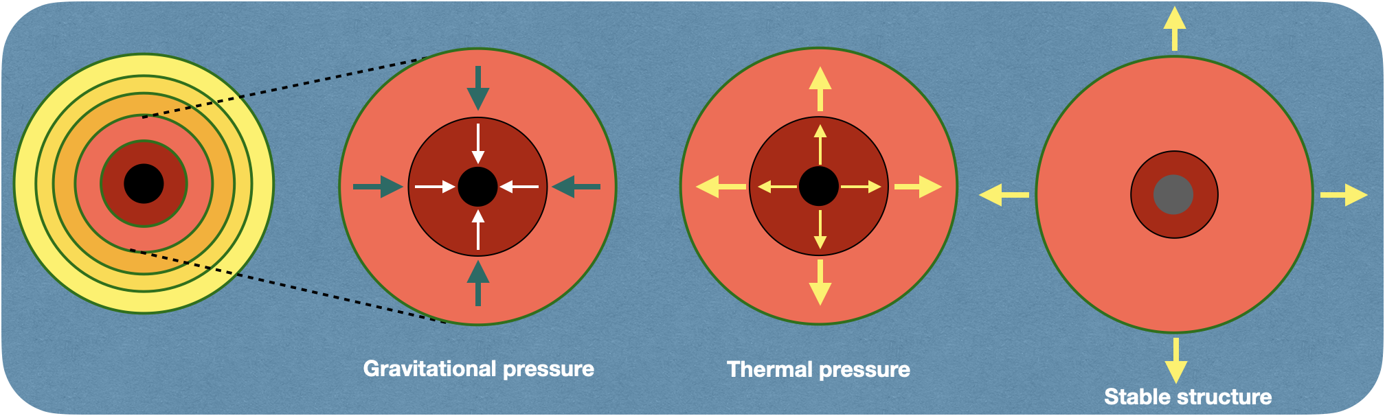
Table of Contents
- Category: About
- Resources: at GitHub
- Project URL: Go to the repository
- Reference
Introduction
Gravitational collapse is a fascinating and complex phenomenon in astrophysics that occurs when a massive object, such as a star, reaches the end of its life cycle. It involves the force of gravity overpowering other forces, leading to the object's collapse under its own gravitational pull.
- Equilibrium and Stability: Stars achieve equilibrium through a balance between the gravitational force pulling inwards and the pressure (thermal or radiation pressure) pushing outwards. This equilibrium is crucial for the star to maintain a stable size and shape throughout most of its life.
- Conditions for Gravitational Collapse: When a massive star exhausts its nuclear fuel, it can no longer produce the energy necessary to maintain the pressure that counteracts gravity. Depending on the mass of the star, various outcomes can occur, such as supernovae, neutron stars, or black holes.
- Hydrostatic Equilibrium Equation: The equilibrium of a star is governed by the hydrostatic equilibrium equation, which relates the pressure gradient to the mass density and gravitational force:
$$ \frac{dP}{dr} = - \frac{G M(r) \rho(r)}{r^2} $$
where,
- P = Pressure inside the star,
- r = Radial distance from the center of the star
- G = Gravitationa; constant
- M(r) = Mass enclosed within the radius r
- ρ(r) Mass desnity at the radial distance
- Equation of State: The equation of state describes the relationship between the pressure, density, and temperature within the star. Different equations of state apply to different stages of a star's life, and they play a significant role in determining its fate during collapse.
- Chandrasekhar Limit: For stars supported by electron degeneracy pressure (white dwarfs), there is a maximum mass known as the Chandrasekhar limit. If a white dwarf exceeds this limit (approximately 1.4 times the mass of the Sun), it can no longer maintain electron degeneracy pressure and may undergo a type Ia supernova.
- Schwarzschild RadiusIf the core of a massive star has a mass greater than the Tolman-Oppenheimer-Volkoff (TOV) limit, it will undergo a catastrophic gravitational collapse. The critical size at which a body becomes a black hole is given by the Schwarzschild radius:
$$R_s = \frac{2 G M}{c^2}$$
where,
- Rs = Schwarschild radius
- M = mass of the objects
- c = speed of light in a vacuum.
- General Relativit: In the final stages of a massive star's collapse, General Relativity becomes essential to describe the extreme curvature of spacetime near the core, especially when a black hole forms.
- Numerical Simulations: Due to the complexity of gravitational collapse, numerical simulations using computational methods like hydrodynamics and numerical relativity are crucial for studying the detailed behavior of collapsing stars and the formation of black holes.
Studying gravitational collapse is a deeply intricate and mathematically demanding field. Astrophysicists use sophisticated mathematical models, equations, and simulations to gain a deeper understanding of this phenomenon and its consequences in the universe.
Monte Carlo simulation
Monte Carlo simulation is a powerful numerical method used in various scientific and engineering fields, including astrophysics. It's particularly useful for tackling complex problems involving random or probabilistic processes, such as gravitational collapse. Let's outline the steps you can follow to learn and implement Monte Carlo simulations for studying gravitational collapse:
- Step 1: Understand the Basics of Monte Carlo Simulation: Familiarize yourself with the fundamental concepts of Monte Carlo simulation, including random sampling, probability distributions, and the Law of Large Numbers. Understanding these principles is crucial for effectively applying the method.
- Step 2: Choose a Gravitational Collapse Model: Decide on the type of gravitational collapse you want to study. It could be the final stages of a massive star's collapse leading to a black hole formation or other specific scenarios relevant to your research interest.
- Step 3: Define the Physical Model: Formulate the physical model of the gravitational collapse you want to simulate. This includes specifying the equations of state, hydrostatic equilibrium equations, and other relevant physics involved in the process.
- Step 4: Discretize the System: Transform the continuous physical model into a discrete representation suitable for Monte Carlo simulations. This involves dividing the physical space into cells or grid points and approximating the continuous equations on these discrete points.
- Step 5: Implement the Monte Carlo Simulation: Write code to perform the Monte Carlo simulation. You'll need to randomly sample initial conditions (mass, density, temperature, etc.) from probability distributions that represent the uncertainty and randomness in the system. Then, evolve the system over time using random walks or other probabilistic methods.
- Step 6: Handle the Gravitational Interaction: In gravitational collapse, the force of gravity plays a central role. You'll need to incorporate the gravitational interaction between particles (representing mass elements) in your simulation. One common approach is to use Newton's law of gravity to calculate the forces between particles.
- Step 7: Consider Stellar Evolution: If your study involves stellar collapse, you'll need to consider the evolution of the star leading up to the collapse. This can include accounting for nuclear burning stages, mass loss, and changes in the equation of state as the star evolves.
- Step 8: Analyze Simulation Results: Run the Monte Carlo simulation for a sufficient number of iterations to obtain statistically meaningful results. Analyze the data to understand the behavior of the collapsing system, identify interesting features, and draw conclusions about the gravitational collapse process.
- Step 9: Validate and Refine the Model: Validate your Monte Carlo model against known analytical solutions or observational data, where possible. If discrepancies arise, refine your model or numerical methods accordingly.
Gravitational collapse is a complex topic, and Monte Carlo simulations are just one approach to study it. Continue learning about other numerical techniques, such as hydrodynamics and numerical relativity, to expand your knowledge and improve your understanding of the phenomenon.
1D Monte Carlo simulation of particles undergoing gravitational collapse
import numpy as np
import matplotlib.pyplot as plt
# Constants
G = 6.67430e-11 # Gravitational constant (m^3 kg^(-1) s^(-2))
M_sun = 1.989e30 # Mass of the Sun (kg)
R_sun = 6.957e8 # Radius of the Sun (m)
# Parameters
num_particles = 1000
mass_range = (0.5 * M_sun, 100 * M_sun) # Mass range of particles
initial_density_range = (100, 500) # Initial density range of particles (kg/m^3)
initial_velocity_range = (0, 100) # Initial velocity range of particles (m/s)
total_time = 1.0e3 # Total simulation time (s)
time_step = 1.0e2 # Time step (s)
def initialize_particles():
masses = np.random.uniform(mass_range[0], mass_range[1], num_particles)
densities = np.random.uniform(initial_density_range[0], initial_density_range[1], num_particles)
velocities = np.random.uniform(initial_velocity_range[0], initial_velocity_range[1], num_particles)
return masses, densities, velocities
def calculate_gravitational_force(mass1, mass2, distance):
return G * mass1 * mass2 / distance**2
def update_particle_positions(positions, velocities, time_step):
return positions + velocities * time_step
def main():
masses, densities, velocities = initialize_particles()
positions = np.zeros(num_particles)
time = 0
while time < total_time:
for i in range(num_particles):
# Update positions
positions[i] = update_particle_positions(positions[i], velocities[i], time_step)
# Calculate net force on the particle due to gravitational interaction with others
net_force = 0.0
for j in range(num_particles):
if i != j:
distance = np.abs(positions[i] - positions[j])
force = calculate_gravitational_force(masses[i], masses[j], distance)
net_force += force
# Update velocities based on the net force
acceleration = net_force / masses[i]
velocities[i] += acceleration * time_step
time += time_step
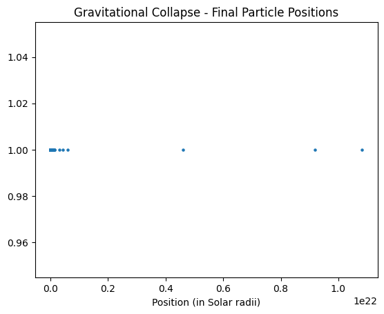
# Plot the final positions of the particles
plt.scatter(positions / R_sun, np.ones(num_particles), marker='o', s=5)
plt.xlabel('Position (in Solar radii)')
plt.title('Gravitational Collapse - Final Particle Positions')
plt.show()
if __name__ == "__main__":
main()
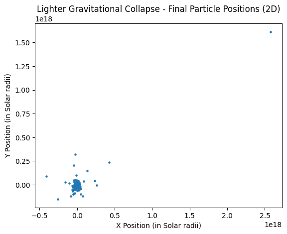
2D Monte Carlo simulation of gravitational collapse:
In this case, we will consider particles moving in a two-dimensional plane under the influence of gravitational forces. The rest of the code structure will remain similar, but we'll update the functions to handle two-dimensional positions and velocities.
              import numpy as np
            import matplotlib.pyplot as plt

            # Constants
            G = 6.67430e-11    # Gravitational constant (m^3 kg^(-1) s^(-2))
            M_sun = 1.989e30    # Mass of the Sun (kg)
            R_sun = 6.957e8     # Radius of the Sun (m)

            # Parameters
            num_particles = 1000  # Reducing the number of particles for lighter simulation
            mass_range = (0.5 * M_sun, 100 * M_sun)
            initial_density_range = (100, 500)
            initial_velocity_range = (0, 100)
            total_time = 1.0e4    # Reducing the total simulation time
            time_step = 1.0e1     # Reducing the time step

            def initialize_particles():
                masses = np.random.uniform(mass_range[0], mass_range[1], num_particles)
                densities = np.random.uniform(initial_density_range[0], initial_density_range[1], num_particles)
                velocities = np.random.uniform(initial_velocity_range[0], initial_velocity_range[1], size=(num_particles, 2))
                return masses, densities, velocities

            def calculate_gravitational_force(mass1, mass2, distance):
                return G * mass1 * mass2 / distance**2

            def update_particle_positions(positions, velocities, time_step):
                return positions + velocities * time_step

            def main():
                masses, densities, velocities = initialize_particles()
                positions = np.zeros((num_particles, 2))
                time = 0

                while time < total_time:
                    for i in range(num_particles):
                        # Update positions
                        positions[i] = update_particle_positions(positions[i], velocities[i], time_step)

                        # Calculate net force on the particle due to gravitational interaction with others
                        differences = positions - positions[i]
                        distances = np.linalg.norm(differences, axis=1)
                        distances[i] = 1.0  # Set distance to self to avoid division by zero
                        forces = calculate_gravitational_force(masses[i], masses, distances)
                        net_force = np.sum((forces / distances)[:, np.newaxis] * differences, axis=0)

                        # Update velocities based on the net force
                        acceleration = net_force / masses[i]
                        velocities[i] += acceleration * time_step

                    time += time_step

                # Plot the final positions of the particles
                plt.scatter(positions[:, 0] / R_sun, positions[:, 1] / R_sun, marker='o', s=5)
                plt.xlabel('X Position (in Solar radii)')
                plt.ylabel('Y Position (in Solar radii)')
                plt.title('Lighter Gravitational Collapse - Final Particle Positions (2D)')
                plt.show()

            if __name__ == "__main__":
                main()
Machine learning Algorithm in Electromagnetic algorithms
The EM algorithm is used for obtaining maximum likelihood estimates of parameters when some of the data is missing. The details on the Maximum likelihood can be found in Maximum Likelihood Estimation (MLE) in python.
This note is provided by Martin Haugh and link is: The EM algorithms.
References
- Monte carlo simulation fundamentals on github repository.
- My notes on Monte Carlo simulation on my lecture note website.
- Gravitational Collapse A. Beesham & S. G. Ghosh
- Gravitational-collapse, W. B. BONNOR
- GitHub repo on gravitational collapse.
- Gravitational Collapse of Rotating Bodies Jeffrey M. Cohen
Some other interesting things to know:
- Visit my website on For Data, Big Data, Data-modeling, Datawarehouse, SQL, cloud-compute.
- Visit my website on Data engineering