𝑬𝒏𝒔𝒆𝒎𝒃𝒍𝒆 𝑳𝒆𝒂𝒓𝒏𝒊𝒏𝒈 𝒊𝒏 𝑫𝒂𝒕𝒂 𝑺𝒄𝒊𝒆𝒏𝒄𝒆
Content
Introduction
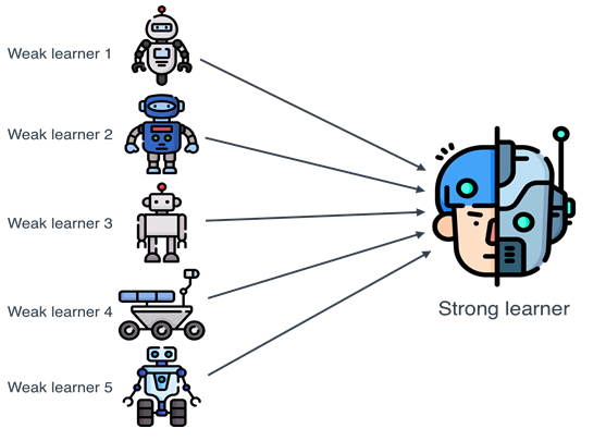
Ensemble learning in machine learning refers to techniques that combine the predictions from multiple models (learners) to improve the overall performance. The main idea is that a group of weak learners (models with moderate accuracy) can come together to form a strong learner. Ensemble methods can often achieve better results than individual models by reducing variance, bias, or improving predictions.
Ensemble Techniques in Machine Learning: Here are some of the most commonly used ensemble techniques:
- Bagging (Bootstrap Aggregating)
- Boosting
- Stacking (Stacked Generalization)
- Blending
These ensemble techniques can significantly improve the accuracy and robustness of machine learning models by leveraging the strengths of multiple models. However, it’s important to note that ensemble methods may come at the cost of interpretability, as the final model becomes more complex.
Algorithms for Ensemble Learning:
- Random Forest
- Voting
- Gradient Boosting Machines (GBMs)
- XGBoost, LightGBM, and CatBoost
- Bagging Variants
Different type ensemble methods
There are several types of ensemble methods, each with its own strengths and weaknesses.
1. Bagging (Bootstrap Aggregating)
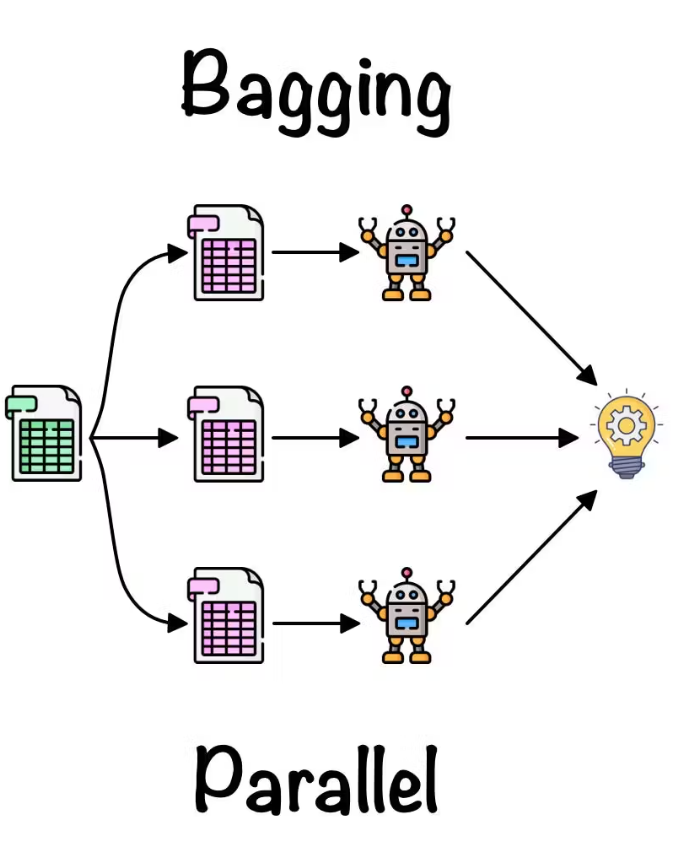
Bagging involves creating multiple models from a single base model by training each model on a different subset of the training data. The subsets are created using bootstrap sampling, where samples are drawn from the original dataset with replacement. Each base model is trained independently, and their predictions are combined using majority voting for classification or averaging for regression. Random Forest is a popular example of a bagging algorithm that uses decision trees as base models.Let’s assume we have \( B \) models \( f_1(x), f_2(x), \dots, f_B(x) \), each trained on a bootstrap sample of the data. The final ensemble prediction \( \hat{f}(x) \) is:
- For regression: \[ \hat{f}(x) = \frac{1}{B} \sum_{i=1}^{B} f_i(x) \]
- For classification: \[ \hat{f}(x) = \text{mode}(f_1(x), f_2(x), \dots, f_B(x)) \]

2. Boosting
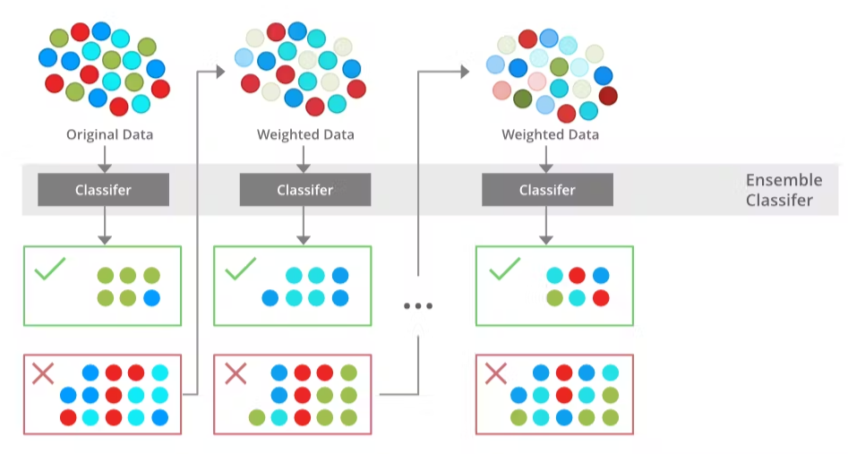
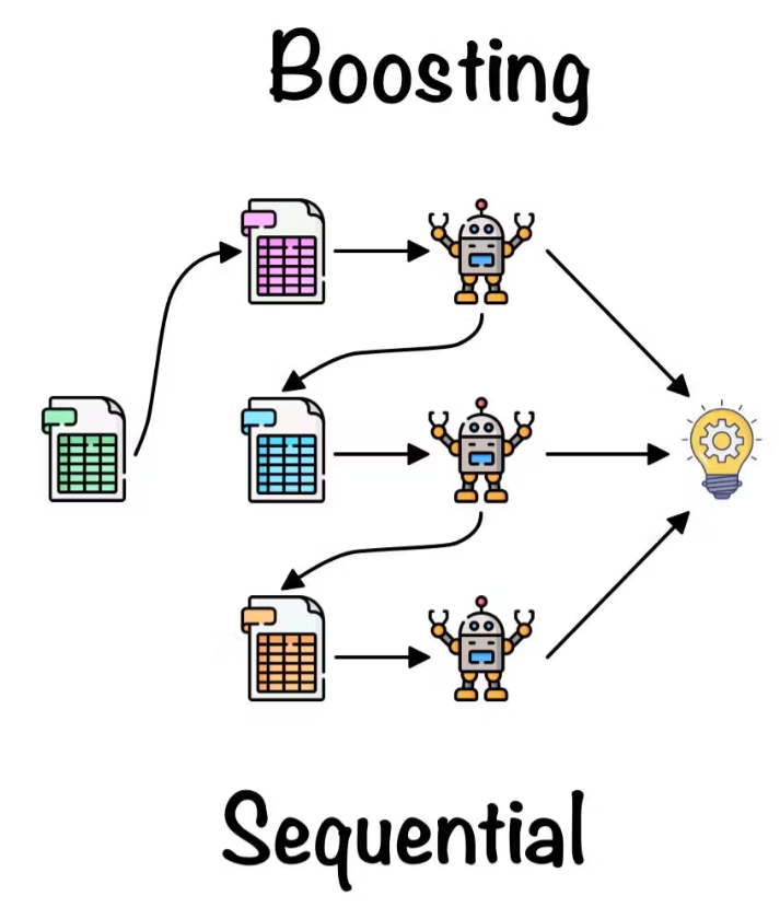
Boosting is an iterative process where weak learners (base models) are trained sequentially, with each subsequent model focusing on the mistakes made by the previous models. The most well-known boosting algorithm is AdaBoost (Adaptive Boosting), which adjusts the weights of the training samples based on the performance of the previous models. Gradient Boosting is another popular boosting technique that uses gradient descent to minimize the loss function and improve the ensemble’s performance.
In AdaBoost, each model is assigned a weight, and misclassified points are given more weight in the next iteration. Assume we have \( B \) weak learners, \( f_1(x), f_2(x), \dots, f_B(x) \), each assigned a weight \( \alpha_i \).
The final model is a weighted sum of all weak learners:
\[ \hat{f}(x) = \text{sign}\left( \sum_{i=1}^{B} \alpha_i f_i(x) \right) \] Here, \( \alpha_i \) is calculated based on the error rate of each weak learner.
3. Stacking (Stacked generation)
Stacking involves training multiple base models on the same dataset and then using a meta-model to combine their predictions. The base models are trained independently, and their outputs are used as features for the meta-model. The meta-model is trained to learn the optimal way to combine the predictions of the base models. Stacking can handle heterogeneous base models, allowing for different types of machine-learning algorithms.Let \( f_1(x), f_2(x), \dots, f_B(x) \) be the base models. The meta-model \( g(x) \) takes the predictions of these base models as input:
\[ \hat{f}(x) = g(f_1(x), f_2(x), \dots, f_B(x)) \]The goal is for the meta-model to learn how to best combine the base models’ predictions.
4. Random Forest
A Random Forest is an extension of the bagging technique, where multiple decision trees are used as the base learners. The key difference from bagging is that Random Forest introduces additional randomness by selecting a random subset of features at each split in the decision trees. Here are key points about Random Forest:- Random Forest involves creating multiple decision trees by selecting random subsets of features and data points to build each tree.
- Each tree in the forest is trained independently, and the final prediction is made by aggregating the predictions of all trees through voting or averaging.
- This algorithm is known for its robustness against overfitting and its ability to handle high-dimensional data effectively.
- Random Forest is widely used in various applications due to its simplicity, scalability, and high accuracy in both classification and regression tasks.
Assume we have \( B \) decision trees \( T_1(x), T_2(x), \dots, T_B(x) \), each trained on different bootstrap samples and a random subset of features. The final prediction is:
- For regression: \[ \hat{f}(x) = \frac{1}{B} \sum_{i=1}^{B} T_i(x) \]
- For classification: \[ \hat{f}(x) = \text{mode}(T_1(x), T_2(x), \dots, T_B(x)) \]
5. Voting
Voting is an ensemble method where multiple models (either of the same type or different types) are trained on the same dataset, and their predictions are combined using voting for classification tasks or averaging for regression tasks.- Hard Voting: The final prediction is the majority vote among the models.
- Soft Voting: Each model outputs a probability, and the final prediction is based on the weighted sum of these probabilities.
Let \( f_1(x), f_2(x), \dots, f_B(x) \) represent \( B \) models.
- For hard voting (classification): \[ \hat{f}(x) = \text{mode}(f_1(x), f_2(x), \dots, f_B(x)) \]
- For soft voting (classification with probabilities \( p_1, p_2, \dots, p_B \)): \[ \hat{f}(x) = \text{argmax} \left( \sum_{i=1}^{B} w_i p_i(x) \right) \] where \( w_i \) is the weight assigned to the \( i \)-th model.
6. Blending
Blending is similar to stacking, but the key difference is how the meta-model is trained. In stacking, the base models are trained using cross-validation, and their predictions are passed to the meta-model. In blending, a holdout validation set is used for training the meta-model, and the base models are trained on the entire training set.These ensemble techniques can significantly improve the accuracy and robustness of machine learning models by leveraging the strengths of multiple models. However, it’s important to note that ensemble methods may come at the cost of interpretability, as the final model becomes more complex.
Let the training set be split into two parts:
- Training set for base models: \( X_{\text{train}} \)
- Holdout validation set for meta-model: \( X_{\text{holdout}} \)
Train base models \( f_1(x), f_2(x), \dots, f_B(x) \) on \( X_{\text{train}} \).
Train a meta-model \( g(x) \) on the predictions of these base models on \( X_{\text{holdout}} \):
\[ \hat{f}(x) = g(f_1(x), f_2(x), \dots, f_B(x)) \]7. Gradient Boosting Machines (GBMs)
Gradient Boosting is an extension of boosting that optimizes a differentiable loss function by iteratively adding weak learners (typically decision trees) that fit the residual errors of the previous model.Mathematical explanantion:
- Initialize the model with a constant value: \[ F_0(x) = \arg \min_{\gamma} \sum_{i=1}^{n} L(y_i, \gamma) \] where \( L \) is the loss function and \( y_i \) are the true labels.
- For each iteration \( m = 1, 2, \dots, M \):
- Compute the residuals (error) \( r_i^{(m)} \) of the current model: \[ r_i^{(m)} = -\left[ \frac{\partial L(y_i, F(x_i))}{\partial F(x_i)} \right]_{F(x) = F_{m-1}(x)} \]
- Train a weak learner \( h_m(x) \) to fit the residuals.
- Update the model by adding the weak learner to the current model: \[ F_m(x) = F_{m-1}(x) + \eta h_m(x) \] where \( \eta \) is the learning rate.
- The final prediction is \( F_M(x) \), the sum of all weak learners.
8. XGBoost, LightGBM, and CatBoost
These are highly optimized and scalable implementations of Gradient Boosting, each offering its own improvements:- XGBoost uses regularization to reduce overfitting.
- LightGBM focuses on efficiency by using a leaf-wise tree growth strategy.
- CatBoost is optimized for categorical features and reduces overfitting through feature combination techniques.
9. Bagging Variants
Pasting is a variant of bagging where instead of bootstrap sampling (sampling with replacement), we sample subsets of the training data without replacement. It reduces variance in a slightly different way compared to standard bagging.If we have \( N \) training examples, instead of sampling with replacement to create different training sets, we sample without replacement, ensuring all training examples are used only once in each subset.
Each method has its own strengths, and the choice of the ensemble method often depends on the specific problem at hand, dataset characteristics, and desired trade-offs between bias, variance, and computational cost.
References
Some other interesting things to know:
- Visit my website on For Data, Big Data, Data-modeling, Datawarehouse, SQL, cloud-compute.
- Visit my website on Data engineering

