Polynomial regression is a statistical technique for modeling a relationship between a dependent variable
() and one or more independent variables () using a polynomial function. In other words, it is a way of fitting a curve to a set of data points.
The general form of the polynomial regression model is:
$$y = \beta_0 +\beta_1 x +\beta_2 x^2 + .... \beta_n x^n$$
where,
= is the dependent variable.
is the independent variable.
are the coefficients of the polynomial terms.
The degree of the polynomial is determined by the highest power of , denoted as .
For example, a polinomial of degree 2 is quadratic equation, and a polinomial of degree 3 is a cubic equation.
Fitting a polynomial regression model
The goal of polynomial regression is to fit the polinomial curve to the data in a way that minimizes the sum of squared differences between the observed and predicted values i.e. RSS.
The RSS is a measure of the error between the predicted values of y and the actual values of y.
The equation for a simple linear regression (degree 1) is a special case of polynomial regression, where n =1.
$$y = \beta_0 +\beta_1 x$$
The coefficients
are typically estimated using methods such as the method of least squares. The model is then used to make predictions based on new values of
.
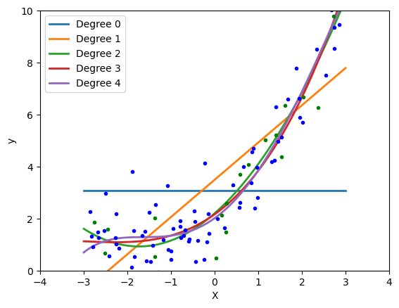
It's important to note that while polynomial regression allows for a more flexible fit to the data, it also runs the risk of overfitting, especially with higher-degree polynomials. Overfitting occurs when the model captures noise or fluctuations in the training data, leading to poor generalization to new, unseen data.
There are two main methods for fitting polynomial regression models:
Least squares: This is the most common method for fitting polynomial regression models. It uses an iterative algorithm to find the coefficients that minimize the RSS.
Regularization: This method can be used to prevent overfitting, which occurs when a model fits the training data too well and does not generalize well to new data. There are several different regularization methods, but the most common is ridge regression.
Interpreting the coefficients
The coefficients of a polynomial regression model can be interpreted in the following way:
is the average value of y
is the slope of the line or curve at the point (0, )
is the rate of change of the slope
is the rate of change of the rate of change
...
Applications of polynomial regression
Polynomial regression has a wide variety of applications, including:
Predicting sales: Polynomial regression can be used to predict sales based on factors such as price, advertising, and economic conditions.
Modeling the growth of plants: Polynomial regression can be used to model the growth of plants based on factors such as temperature, sunlight, and nutrients.
Analyzing financial data: Polynomial regression can be used to analyze financial data to identify trends and patterns.
Improving the accuracy of machine learning models: Polynomial regression can be used to improve the accuracy of machine learning models by providing them with a more complex and flexible representation of the data.
Example-1
Importing the libraries:
                    # import libraries
                    import numpy as np
                    import pandas as pd
                    import matplotlib.pyplot as plt
                    %matplotlib inline
Generating datasets/ loading the datasets:
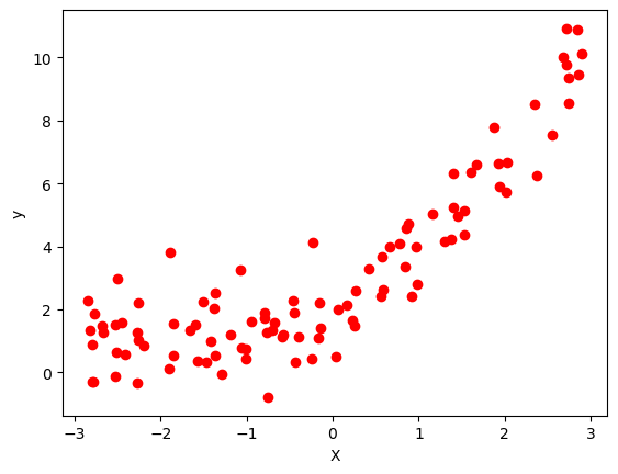
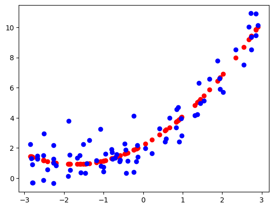
In our current example, we generate a random dataset for X and y. Specially in our current example, we have considered following equation to generate the random data for y:
$$y = \frac{1}{2} x^2 +\frac{3}{2} x +2 +\text{outliers}$$
and hence python code is:
                X = 6 * np.random.rand(100,1)-3
                y = 0.5*X**2 + 1.5*X + 2 + np.random.randn(100,1)

                # quadratic equation is shown above

                plt.scatter(X, y, color='r')
                plt.xlabel("X")
                plt.ylabel("y")
                plt.show()
which gives the data for our example and plot the generated datasets.
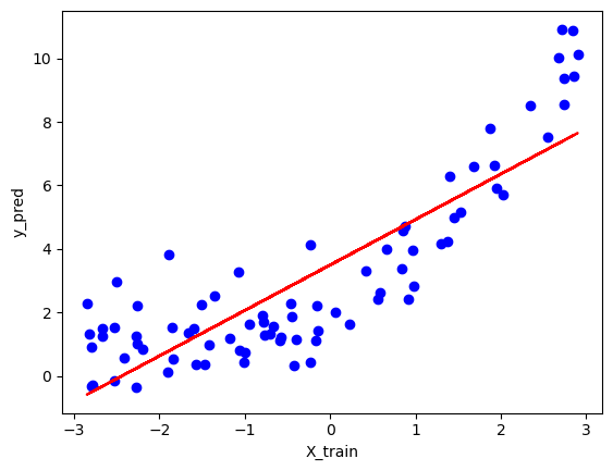
Simple line:Now let's start with the simple line which is actually case of degree=1
## Apply linear regression
from sklearn.linear_model import LinearRegression
regression1 = LinearRegression()
regression1.fit(X_train, y_train)
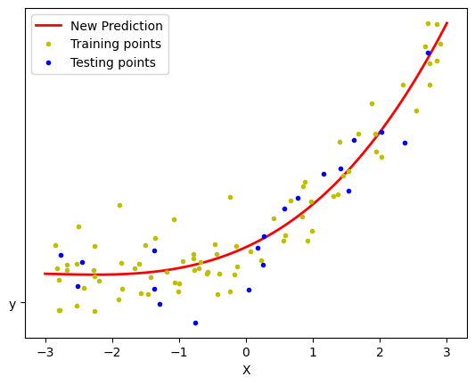
## plot Training data plot and best fit line
plt.scatter(X_train, y_train, color = 'b')
plt.plot(X_train, regression1.predict(X_train), color = 'r')
plt.xlabel("X_train")
plt.ylabel("y_pred")
plt.show()
from sklearn.metrics import r2_score
score = r2_score(y_test, regression1.predict(X_test))
print(f"The r-squared value for the model is= {score}")
so it gave The r-squared value for the model is= 0.6405513731105184 and
The coefficient in the case can be obtained using: regression.coef_ = [[1.43280818]].
Quadratic equation:
Next we are going to use following equation:
$$y = \beta_0 +\beta_1 x +\beta_2 x^2$$

 The coefficient in the case can be obtained using: