
Regression Model parameter estimation
Intorduction
- The values of \(\beta_0\), \(\beta_1\), and \(\sigma^2\) will almost never be known to an investigator.
Instead, sample data consists of n observed pairs
(\(x_1\), \(y_1\)), … , (\(x_n \), \(y_n\)),
from which the model parameters and the true regression line itself can be estimated.
The data (pairs) are assumed to have been obtained independently of one another.
where
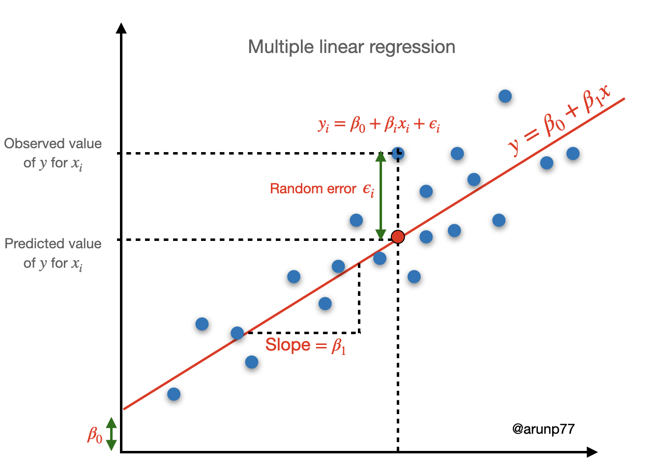
\(Y_i =\beta_0+\beta_1 x_i + \epsilon_i\) for \(i = 1, 2, … , n\)
and the \(n\) deviations \(\epsilon_1, \epsilon_2, ..., \epsilon_n\)
The “best fit” line is motivated by the principle of least squares, which can be traced back to the German mathematician Gauss (1777–1855):
A line provides the best fit to the data if the sum of the squared vertical distances (deviations) from the observed points to that line is as small as it can be.
The sum of squared vertical deviations from the points \((x_1, y_1),…, (x_n, y_n)\) to the line is then:
\(f(b_0, b_1) = \sum_{i=1}^n [y_i - (b_0+b_1 x_i)]^2\)
The point estimates of \(\beta_0\) and \(\beta_1\), denoted by \(\hat{\beta}_0\) and \(\hat{\beta}_1\), are called the least squares estimates they are those values that minimize \(f(b_0, b_1)\).
The fitted regression line or least squares line is then the line whose equation is:
\(y = \hat{\beta}_0+\hat{\beta}_1 x\).
The minimizing values of b0 and b1 are found by taking partial derivatives of \(f(b_0, b_1)\) with respect to both \(b_0\) and \(b_1\), equating them both to zero [analogously to \(fʹ(b) = 0\) in univariate calculus], and solving the equations
\(\frac{\partial f(b_0, b_1)}{\partial b_0} = \sum 2 (y_i - b_0 - b_1 x_i) (-1) = 0\)
\(\frac{\partial f(b_0, b_1)}{\partial b_1} = \sum 2 (y_i - b_0 - b_1 x_i) (-x_i) = 0\).
Which in term gives two equations:
\(\sum (y_i - b_0 - b_1 x_i) = 0\)
\(\sum (y_i x_i- b_0x_i - b_1 x_i^2) = 0\).
after some simplification, we can get
\(\boxed{b_1 = \hat{\beta}_1 = \frac{\sum (x_i - \bar{x})(y_i - \bar{y})}{\sum (x_i - \bar{x})^2} = \frac{S_{xy}}{S_{xx}}}\)
where
- \(S_{xy}= \sum x_i y_i - \frac{\sum x_i \sum y_i}{n}\)
- \(S_{xx} = \sum x_i^2 - \frac{\sum x_i^2}{n}\)
(Typically columns for \(x_i, y_i, x_i y_i\) and \(x_i^2\) and constructed and then \(S_{xy}\) and \(S_{xx}\) are calculated.)
The least squares estimate of the intercept \(\beta_0\) of the true regression line is
\(\boxed{b_0 = \hat{\beta}_0 = \frac{\sum y_i - \hat{\beta}_1 \sum x_i}{n} = \bar{y}- \hat{\beta}_1 \bar{x}}\).
The computational formulas for \(S_{xy}\) and \(S_{xx}\) require only the summary statistics \(\sum x_i, \sum y_i, \sum x_i y_i\) and \(\sum x_i^2\) (\(\sum y_i^2\) will be needed shortly for the variance.)
Fitted values
1. Fitted values
The fitted (or predicted) values \(\hat{y}_1\), \(\hat{y}_2\), ...., \(\hat{y}_n\) are obtained by substituting \(x_1, x_2, ...., x_n\) into the equation of the estimated regression line:
- \(\hat{y}_1 = \hat{\beta}_0 + \hat{\beta}_1 x_1\)
- \(\hat{y}_2 = \hat{\beta}_0 + \hat{\beta}_1 x_1\)
- .
- .
- .
- \(\hat{y}_n = \hat{\beta}_0 + \hat{\beta}_1 x_n\)
2. Residuals
- The differences \(y_1 - \hat{y}_1\), \(y_2 - \hat{y}_2\), ....., \(y_n - \hat{y}_n\) between the observed and fittted \(y\) values.
When the estimated regression line is obtained via the principle of least squares, the sum of the residuals should in theory be zero, if the error distribution is symmetric, since
\(\sum (y_i - (\hat{\beta}_0+ \hat{\beta}_1 x_i)) = n \bar{y}- n \hat{\beta}_0 - \hat{\beta}_1 n \bar{x} = n \hat{\beta}_0 - n \hat{\beta}_0 = 0\).
- \(y_i-\hat{y}_i > 0 \Rightarrow \) if the point \((x_i y_i)\) lies above the line
- \(y_i-\hat{y}_i <> 0 \Rightarrow \) if the point \((x_i y_i)\) lies below the line
The residual can be thought of as a measure of deviation and we can summarize the notation in the following way:
\(Y_i - \hat{Y}_i = \hat{\epsilon}_i\)
3. Estimating \(\sigma^2\) and \(\sigma\)
The parameter \(\sigma^2\) determines the amount of spread about the true regression line.
An estimates of \(\sigma^2\) will be used in confidence interval (CI)formulas and hypothesis-testing procedures presented in the next two sections.
- Many large deviations (residuals) suggest a large value of \(\sigma^2\), whereas deviations all of which are small in magnitude suggest that \(\sigma^2\) is small.
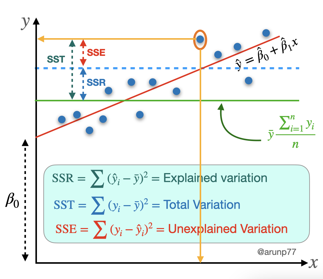
Error sum of squares (SSE): The error sum of squares SSE can be interpreted as a measure of how much variation in y is left unexplained by the model—that is, how much cannot be attributed to a linear relationship.
The SSE (equivalently, residual sum of squares), denoted by SSE is:
\(\boxed{{\rm SSE} = \sum (y_i - \hat{y}_i)^2 = \sum [y_i - (\hat{\beta}_0+\hat{\beta}_1 x_i)]^2}\)
and the estimates of \(\sigma^2\) is
\(\hat{\sigma}^2 =s^2 = \frac{\text{SSE}}{n-2} = \frac{\sum (y - \hat{y}_i)^2}{n-2} = \frac{1}{n-2} \sum_{i=1}^n \hat{e}_i^2\).
(Note that the homoscedasticity assumption comes into play here).
The divisor \(n – 2\) in \(s^2\) is the number of degrees of freedom \((df)\) associated with SSE and the estimate \(s^2\).
- This is because to obtain \(s^2\), the two parameters \(\beta_0\) and \(\beta_1\) must first be estimated, which results in a loss of \(2\) \(df\) (just as \(\mu\) had to be estimated in one sample problems, resulting in an estimated variance based on \(n – 1\) df in our previous t-tests).
Computation of SSE from the defining formula involves much tedious arithmetic, because both the predicted values and residuals must first be calculated.

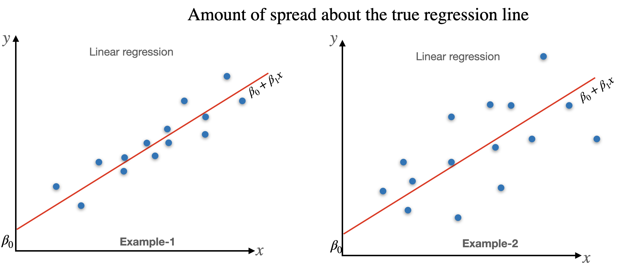
The points in the first plot all fall exactly on a straight line. In this case, all (\(100\%\)) of the sample variation in y can be attributed to the fact that x and y are linearly related in combination with variation in x.
The points in the second plot do not fall exactly on a line, but compared to overall y variability, the deviations from the least squares line are small.
It is reasonable to conclude in this case that much of the observed y variation can be attributed to the approximate linear relationship between the variables postulated by the simple linear regression model.
- When the scatter plot looks like that in the third plot, there is substantial variation about the least squares line relative to overall y variation, so the simple linear regression model fails to explain variation in y by relating y to x.
In the first plot SSE = 0, and there is no unexplained variation, whereas unexplained variation is small for second, and large for the third plot.
4. Total sum of squares (SST) or Total Variation
A quantitative measure of the total amount of variation in observed y values is given by the total sum of squares.
\(\boxed{{\rm SST} = S_{yy} = \sum (y_i -\bar{y})^2 = \sum y_i^2 - \frac{(\sum y_i)^2}{n}}\).
The SST is the sum of squared deviations about the sample mean of the observed y values – when no predictors are taken into account
4.1. Difference between SST and SSE:
The SST in some sense is as bad as SSE can get if there is no regression model (i.e., slope is 0) then
\(\hat{\beta}_0 = \bar{y}- \hat{\beta}_1 \bar{x} \Rightarrow \hat{y} = \hat{\beta}_0+\underbrace{\hat{\beta}_1}_{=0} \bar{x} = \hat{\beta}_0 = \bar{y}\)
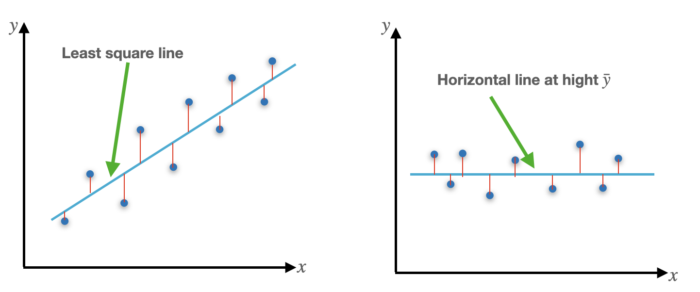
The SSE < SST unless the horizontal line itself is the least square line.
5. Coefficient of determination (\(r^2\))
\(\boxed{r^2 = 1- \frac{{\rm SSE}}{{\rm SST}}} \Rightarrow \) (a number between 0 and 1.)
- The ratio SSE/SST is the proportion of total variation that cannot be explained by the simple linear regression mode and \(r^2\) is the proportion of the observed \(y\) variation explained by the model.
- It is interpreted as the proportion of observed y variation that can be explained by the simple linear regression model (attributed to an approximate linear relationship between y and x).
- The higher the value of \(r^2\), the more successful is the simple linear regression model in explaining y variation.
6. Regression sum of squares (SSR)
The coefficient of determination can be written in a slightly different way by introducing a third sum of squares—regression sum of squares, SSR—given by:
\(\boxed{{\rm SSR} = \sum (\hat{y}_i - \bar{y})^2 = {\rm SST}- {\rm SSE}}\).
Regression sum of squares is interpreted as the amount of total variation that is explained by the model.
Then we have
\(\boxed{r^2 = 1- \frac{{\rm SSE}}{{\rm SST}} = \frac{{\rm SST} - {\rm SSE}}{{\rm SST}} = \frac{{\rm SSR}}{{\rm SST}}} = \frac{\text{Explained Variation}}{\text{Total Variation}}\)
the ratio of explained variation to total variation.
Testing for significance using the slope, \(\beta_1\):
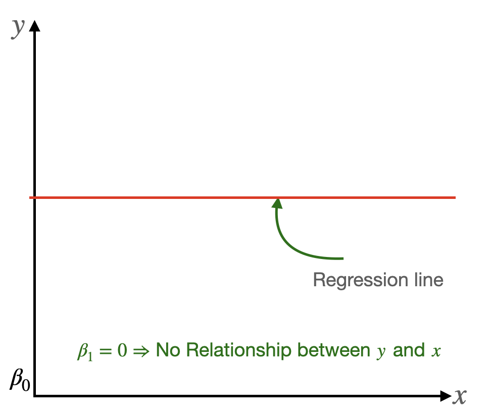
- If \(\beta_1 = 0\), then \(y=\beta_0\), no matter what value \(x\) is.
- Therefore there is no linear relationship between \(x\) and \(y\) when \(\beta_1 = 0\).
Hypothesis test of significance, t-test:
The most commonly encountered pair of hypotheses about \(\beta_1\)
- \(H_0: \beta_1 = 0 \)
\(H_a: \beta_1 \neq 0\).
We are going to see if we have enough evidence to support the alternative hypothesis that the slope is not equal to zero. If we will find a evidence, we will conclude that there is a linear relationship between \(x\) and \(y\).
Here Test statistics: \(\boxed{t=\frac{b_1}{S_{b_1}}}\),
where \(S_{b_1}\) is the standard error for the slope. To calculate this, we use following formula:
\(\boxed{S_{b_1} = \frac{s}{\sqrt{\sum(x_i - \bar{x}_i)^2}}}\),
where \(s = \sqrt{\frac{\text{SSE}}{n-2}}\)
Ways to perform hypothesis testing
There are several ways to check the null and alternative hypotheses when performing hypothesis testing. Here are some common approaches:
Critical Value Approach: The critical value approach involves comparing a test statistic (calculated from the data) to a predetermined critical value based on the chosen significance level (alpha). The steps involved in the critical value approach are as follows:
- Null hypothesis (H0) and alternative hypothesis (Ha) are defined.
- Test statistic (e.g., z-score or t-statistic) is calculated based on the sample data.
- Critical value(s) (denoted as z_crit or t_crit) are determined based on the chosen significance level (alpha) and the distribution of the test statistic.
Comparison: If the test statistic falls within the critical region (i.e.,
- test statistic > critical value for a right-tailed test or
test statistic < critical value for a left-tailed test),
reject the null hypothesis in favor of the alternative hypothesis. Otherwise, if the test statistic falls outside the critical region, fail to reject the null hypothesis.
The critical value approach is commonly used in tests such as z-tests and t-tests, where critical values are obtained from standard tables or calculated based on the desired significance level and the test's distribution.
P-Value Approach: The p-value approach, also known as the probability approach, involves calculating the p-value associated with the observed test statistic. The p-value is the probability of obtaining a test statistic as extreme or more extreme than the observed value, assuming that the null hypothesis is true. The steps involved in the p-value approach are as follows:
- Null hypothesis (H0) and alternative hypothesis (Ha) are defined.
- Test statistic (e.g., z-score or t-statistic) is calculated based on the sample data.
- P-value is calculated, representing the probability of obtaining a test statistic as extreme or more extreme than the observed value, assuming the null hypothesis is true.
- Comparison: If the p-value is less than or equal to the chosen significance level (alpha), reject the null hypothesis in favor of the alternative hypothesis. Otherwise, if the p-value is greater than the significance level, fail to reject the null hypothesis.
The p-value approach provides a measure of the strength of evidence against the null hypothesis. A smaller p-value indicates stronger evidence against the null hypothesis, suggesting that the observed data is unlikely to occur if the null hypothesis is true. The p-value approach allows for more flexibility in choosing significance levels and can be used with a wide range of statistical tests.
Confidence Interval Approach:
- Test statistic and its standard error are calculated based on the sample data.
- Confidence interval is constructed around the test statistic, typically using the formula: test statistic ± (critical value * standard error).
- Comparison: If the null hypothesis value falls outside the confidence interval, reject the null hypothesis. Otherwise, if the null hypothesis value is inside the confidence interval, fail to reject the null hypothesis.
Likelihood Ratio Test:
- Likelihood of the data under the null hypothesis (L(H0)) and alternative hypothesis (L(Ha)) is calculated based on the sample data.
Likelihood ratio is computed as the ratio of the likelihoods:
\(\boxed{\text{likelihood ratio} = \frac{L(Ha)}{L(H0)}}\).
Comparison: If the likelihood ratio is greater than the critical value corresponding to the chosen significance level or if the p-value associated with the likelihood ratio is less than the chosen significance level, reject the null hypothesis. Otherwise, if the likelihood ratio is not greater than the critical value or the p-value is not less than the significance level, fail to reject the null hypothesis.
Bayesian Approach:
- Prior probabilities (P(H0) and P(Ha)) are specified for the null and alternative hypotheses.
Posterior probabilities (P(H0|data) and P(Ha|data)) are calculated using Bayes' theorem:
\(\boxed{P(H0|\text{data}) = \frac{P(H0) * P(\text{data}|H0)}{P(\text{data})}}\) and
\(\boxed{P(Ha|\text{data}) = \frac{P(Ha) * P(\text{data}|Ha)}{P(\text{data})}}\),
where P(data) is the marginal likelihood.
Comparison: Decision is made based on the posterior probabilities, such as comparing P(H0|data) to a threshold. If P(H0|data) is lower than the threshold, reject the null hypothesis. Otherwise, if P(H0|data) is higher than or equal to the threshold, fail to reject the null hypothesis.
Test statistic
1. z-score
- The z-score is used in hypothesis testing when the sample size is large or when the population standard deviation is known.
The formula for calculating the z-score is:
\(\boxed{z = \frac{\bar{x} - μ}{(\sigma / \sqrt{n})}}\),
where \(\bar{x}\) is the sample mean, \(\mu\) is the population mean, \(\sigma\) is the population standard deviation, and \(n\) is the sample size.
The z-score follows a standard normal distribution (mean = 0, standard deviation = 1), allowing for comparison to critical values or calculation of p-values.
2. t-statistic
- The t-statistic is used when the sample size is small and the population standard deviation is unknown.
- The formula for calculating the t-statistic depends on the specific test being performed (e.g., one-sample t-test, independent samples t-test, paired samples t-test).
- The t-statistic follows a t-distribution with degrees of freedom (df) determined by the sample size and the specific test being conducted.
- Comparison to critical values or calculation of p-values is done using the t-distribution
One-Sample t-Test:
The one-sample t-test is used to determine if the mean of a single sample significantly differs from a specified population mean.
The formula for calculating the t-statistic in a one-sample t-test is:
\(\boxed{t = \frac{x-\mu}{s/\sqrt{n}}}\),
where
- \(x\) is the sample mean,
- \(\mu\) is the specified population mean,
- \(s\) is the sample standard deviation, and
- \(n\) is the sample size.
The t-statistic follows a t-distribution with \((n - 1)\) degrees of freedom.
- The null hypothesis (\(H0\)): is that the population mean is equal to the specified value (\(\mu\)), and
- the alternative hypothesis (\(Ha\)): is that the population mean is not equal to \(\mu\).
Independent Samples t-Test:
The independent samples t-test is used to compare the means of two independent groups and determine if they significantly differ from each other.
The formula for calculating the t-statistic in an independent samples t-test is:
\(\boxed{t = \frac{(x_1 - x_2)}{√((s_1^2 / n_1) + (s_2^2 / n_2))}}\),
where
- \(x_1\) and \(x_2\) are the sample means,
- \(s_1\) and \(s_2\) are the sample standard deviations,
- \(n_1\) and \(n_2\) are the sample sizes
of the two groups.
The t-statistic follows a t-distribution with degrees of freedom calculated using a formula that takes into account the sample sizes and variances of the two groups.
- The null hypothesis (\(H0\)): is that the means of the two groups are equal, and
- the alternative hypothesis (\(Ha\)) is that the means are not equal.
Paired Samples t-Test:
The paired samples t-test, also known as the dependent samples t-test, is used to compare the means of two related or paired samples.
The formula for calculating the t-statistic in a paired samples t-test is:
\(\boxed{t = \frac{(\bar{x}_d - \mu_d)}{(s_d / \sqrt{n})}}\),
where
- \(\bar{x}_d\) is the mean difference of the paired observations,
- \(\mu_d\) is the specified population mean difference (usually \(0\) under the null hypothesis),
- \(s_d\) is the standard deviation of the differences, and
- \(n\) is the number of paired observations.
The t-statistic follows a t-distribution with \((n - 1)\) degrees of freedom.
- The null hypothesis (\(H0\)) is that the mean difference is equal to the specified value (\(\mu_d\), often \(0\)), and
- the alternative hypothesis (\(Ha\)) is that the mean difference is not equal to \(\mu_d\).
3. F-Statistic:
- The F-statistic is used in analysis of variance (ANOVA) tests to compare the variability between groups to the variability within groups.
- The formula for calculating the F-statistic depends on the specific ANOVA test being performed (e.g., one-way ANOVA, two-way ANOVA).
- The F-statistic follows an F-distribution with different degrees of freedom for the numerator and denominator, which are determined by the number of groups and sample sizes.
- Comparison to critical values or calculation of p-values is done using the F-distribution.
Analysis of Variance (ANOVA): is a statistical technique used to test for significant differences between the means of two or more groups. ANOVA partitions the total variability in the data into different components to assess the impact of different sources of variation. Here's an explanation of ANOVA with formulas:
- One-Way ANOVA:
- One-Way ANOVA is used when comparing the means of two or more groups on a single independent variable (factor).
The formula for calculating the F-statistic in a one-way ANOVA is:
\(F= \frac{SSB / (k - 1)}{(SSW / (n - k))}\),
where
- \(SSB\) is the between-group sum of squares: \(SSB = \sum n_i (\bar{x}_i-\bar{x})^2\), where \(n_i\) is the sample size of the ith group, \(\bar{x}_i\) is the mean of the ith group, \(\bar{x}\) is the overall mean.
- \(SSW\) is the within-group sum of squares: \(SSW = \sum \sum (x_i - \bar{x}_i)^2\), where \(x_i\) is an individual observation in the ith group, \(\bar{x}_i\) is the mean of the ith group.
- Sometimes, we also need SST = SSB + SSW.
- \(k\) is the number of groups, and
- \(n\) is the total sample size.
- Check example: https://statkat.com/compute-sum-of-squares-ANOVA.php
SSB represents the variability between the group means, and SSW represents the variability within each group.
- The F-statistic follows an F-distribution with \((k - 1)\) numerator degrees of freedom and \((n - k)\) denominator degrees of freedom.
- The null hypothesis (H0): is that the means of all groups are equal, and
- The alternative hypothesis (Ha): is that at least one group mean is different.
- Two-Way ANOVA:
- Two-Way ANOVA is used when comparing the means of two or more groups on two independent variables (factors).
- The formula for calculating the F-statistic in a two-way ANOVA involves multiple sources of variation, including main effects and interaction effects.
- The specific formulas depend on the design of the study (e.g., balanced/unbalanced, fixed/random effects).
- The F-statistic for each effect (main effect or interaction effect) is calculated by dividing the sum of squares for that effect by the corresponding degrees of freedom and mean square error.
- The F-statistics follow an F-distribution with appropriate degrees of freedom.
- The null hypothesis (H0) is that there is no significant effect of the factors or their interaction on the response variable, and
- The alternative hypothesis (Ha) is that there is a significant effect.
4. Chi-Square Statistic:
- The chi-square statistic is used for testing relationships between categorical variables or for testing goodness of fit.
- The formula for calculating the chi-square statistic depends on the specific test being conducted (e.g., chi-square test of independence, chi-square goodness of fit test).
- The chi-square statistic follows a chi-square distribution with degrees of freedom determined by the number of categories or the degrees of freedom associated with the test.
- Comparison to critical values or calculation of p-values is done using the chi-square distribution.
The Chi-Square statistic is a test statistic used in hypothesis testing to assess the relationship between categorical variables or to test for goodness of fit. It compares the observed frequencies with the expected frequencies under a specified hypothesis.
- Chi-Square Test of Independence:
- The Chi-Square test of independence is used to determine if there is a significant association between two categorical variables.
The formula for calculating the Chi-Square statistic in a test of independence is:
\(\chi^2 = \sum \frac{(O-E)^2}{E}\),
where \(\sum\) represents the summation symbol, \(O\) is the observed frequency in each cell of a contingency table, and \(E\) is the expected frequency under the assumption of independence.
- The observed frequencies (\(O\)) are the actual counts of observations in each cell of the contingency table, and the expected frequencie
- (\(E\)) are the counts that would be expected if the two variables were independent.
- The Chi-Square statistic follows a Chi-Square distribution with degrees of freedom calculated based on the number of rows and columns in the contingency table.
- Chi-Square Goodness of Fit Test:
- The Chi-Square goodness of fit test is used to determine if observed categorical data follows a specified distribution or expected frequencies.
The formula for calculating the Chi-Square statistic in a goodness of fit test is:
\(\chi^2 = \sum \frac{(O-E)^2}{E}\),
where \(\sum\) represents the summation symbol, \(O\) is the observed frequency for each category, and \(E\) is the expected frequency under the null hypothesis.
- The observed frequencies (\(O\)) are the actual counts of observations in each category, and the expected frequencies (\(E\)) are the counts that would be expected if the null hypothesis is true.
- The Chi-Square statistic follows a Chi-Square distribution with degrees of freedom determined by the number of categories minus one.
Calculation
To do all these statistics, we may need to find following:
| xi | yi | yi_hat=beta0+beta1*xi | Error | Squared error (yi - yi_hat)^2 | Deviation yi - ybar | Squared Deviation (yi - ybar)^2 |
|---|---|---|---|---|---|---|
| . | . | . | . | . | . | . |
| . | . | . | . | . | . | . |
| . | . | . | . | . | . | . |
| SSE=... | SST=... |
where
- xi =\(x_i\)
- yi = \(y_i\)
- yi_hat = beta0 + beta1 * xi = \(\hat{y}_i = \hat{\beta}_0 + \hat{\beta}_1 x_i\)
- Error (yi - yi_hat)^2 = Error \((y_i - \hat{y}_i)^2\)
- Deviation yi - ybar = Deviation \(y_i - \bar{y}\)
- Squared Deviation (yi - ybar)^2 = Squared deviation \((y_i - \bar{y})^2\(
and
| xi | yi | xi-xbar | yi-ybar | (xi-xbar)(yi-ybar) | (xi-xbar)^2 |
|---|---|---|---|---|---|
| . | . | . | . | . | . |
| . | . | . | . | . | . |
| . | . | . | . | . | . |
to calculate xbar and ybar.
- You can go to following project for a reference for linear regression analysis.
References
- My github Repositories on Remote sensing Machine learning
- A Visual Introduction To Linear regression (Best reference for theory and visualization).
- Book on Regression model: Regression and Other Stories
- Book on Statistics: The Elements of Statistical Learning
- https://www.colorado.edu/amath/sites/default/files/attached-files/ch12_0.pdf
Some other interesting things to know:
- Visit my website on For Data, Big Data, Data-modeling, Datawarehouse, SQL, cloud-compute.
- Visit my website on Data engineering