Introduction

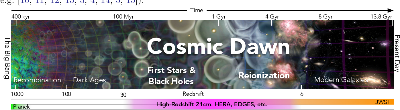
21 cm cosmology is a powerful observational tool to study the early universe, especially during the so-called "Dark Ages" and "Cosmic Dawn" periods, which are difficult to observe by other means. The 21 cm line corresponds to the hyperfine transition of neutral hydrogen (\(H\)) atoms, occurring due to the interaction between the electron's spin and the proton's spin in a hydrogen atom. When the spins flip from parallel to antiparallel, the atom emits a photon with a wavelength of 21 cm (frequency of about 1.42 GHz).

This emission or absorption signal provides crucial information about the physical conditions of the early universe, such as the density of neutral hydrogen, temperature, and the effects of the first stars and galaxies on the intergalactic medium (IGM). It is an essential probe for understanding the "Epoch of Reionization (EoR)", the period when the first stars and galaxies formed and ionized the surrounding hydrogen.

The 21 cm Signal: Key Equations

• \( T_b(z) \): Brightness temperature of the 21 cm signal at redshift \( z \),
• \( x_{\text{HI}} \): Fraction of neutral hydrogen at redshift \( z \),
• \( \delta_b \): Baryon overdensity,
• \( \Omega_b \): Baryon density parameter,
• \( \Omega_m \): Total matter density parameter,
• \( h \): Hubble parameter today (in units of 100 km/s/Mpc),
• \( T_\gamma(z) \): CMB temperature at redshift \( z \),
• \( T_s(z) \): Spin temperature of the neutral hydrogen at redshift \( z \).

Key Terms Explained

1. Spin Temperature \( T_s \): The spin temperature defines the relative population of the two hyperfine levels in neutral hydrogen. It is a weighted combination of three temperatures:
   • Kinetic Temperature \( T_k \): The temperature of the hydrogen gas, governing particle collisions.
   • CMB Temperature \( T_\gamma \): The temperature of the CMB photons interacting with the hydrogen atoms.
   • Lyman-\(\alpha\) Coupling: The interaction of hydrogen atoms with Lyman-\(\alpha\) photons (from the first stars) can also affect the spin temperature.
   The spin temperature is given by: \[ \frac{1}{T_s} = \frac{T_\gamma^{-1} + x_c T_k^{-1} + x_\alpha T_k^{-1}}{1 + x_c + x_\alpha} \] where:
   • \( x_c \): Collision coupling coefficient (proportional to the collision rate between hydrogen atoms),
   • \( x_\alpha \): Wouthuysen-Field effect coupling coefficient, which accounts for the interaction with Lyman-\(\alpha\) photons.
2. Brightness Temperature \( T_b \): The brightness temperature measures the contrast between the 21 cm emission or absorption signal and the background radiation (CMB) at a given redshift. It tells us whether hydrogen is in emission (positive \( T_b \)) or absorption (negative \( T_b \)).

Evolution of the 21 cm Signal in the Early Universe

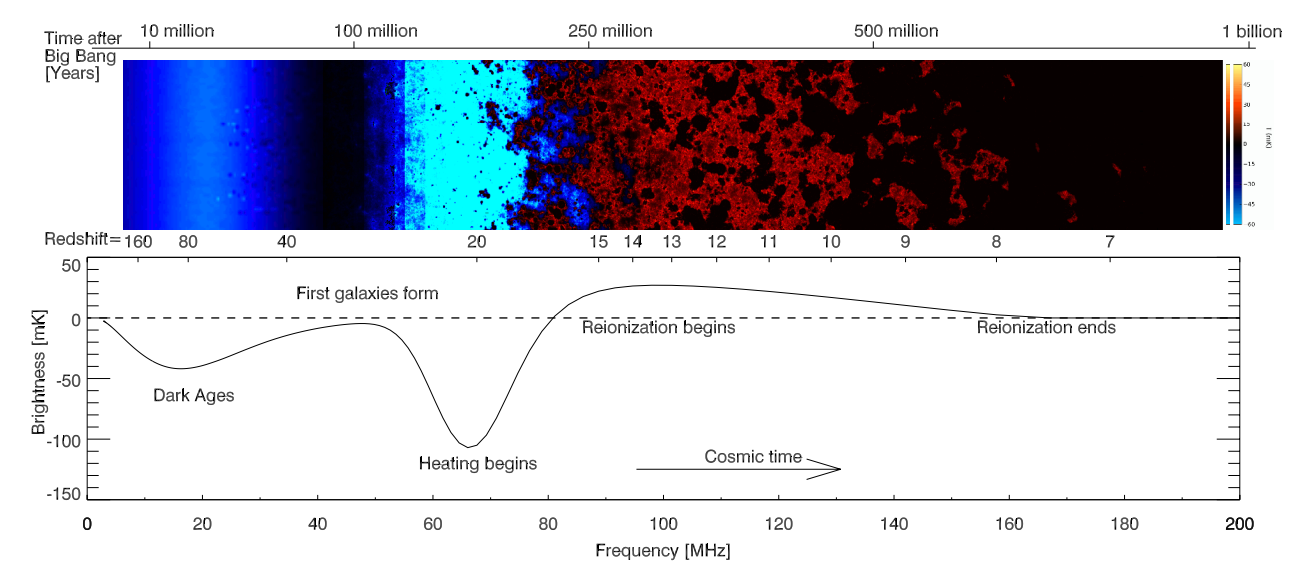
1. Dark Ages (Before Cosmic Dawn, \( z \sim 200 - 30 \)):
   • During the Dark Ages, after recombination but before the first stars form, neutral hydrogen is the dominant component of the IGM.
   • The spin temperature \( T_s \) is in equilibrium with the CMB temperature \( T_\gamma \), so \( T_s \approx T_\gamma \), and there is no observable 21 cm signal since \( T_b = 0 \) (because \( T_s = T_\gamma \)).
   >
2. Cosmic Dawn (Formation of the First Stars, \( z \sim 30 - 15 \)):
   • As the first stars form, they emit Lyman-\(\alpha\) radiation, which decouples the spin temperature \( T_s \) from the CMB via the Wouthuysen-Field effect.
   • The Lyman-\(\alpha\) photons couple the spin temperature \( T_s \) to the kinetic temperature \( T_k \) of the gas.
   • At this stage, \( T_s < T_\gamma \), leading to an absorption signal (negative \( T_b \)).
3. Epoch of Reionization (EoR, \( z \sim 15 - 6 \)):
   • The formation of the first galaxies and quasars ionizes the hydrogen in the IGM.
   • As ionizing radiation increases, neutral hydrogen is depleted, and the 21 cm signal weakens.
   • During reionization, regions of the universe with high neutral hydrogen density will show a mix of emission and absorption signals depending on the local conditions.
   • Eventually, as the universe becomes fully ionized (\( x_{\text{HI}} \rightarrow 0 \)), the 21 cm signal vanishes.

Importance of 21 cm Cosmology

• The formation of the first stars and galaxies,
• The heating of the IGM,
• The timeline of reionization,
• Large-scale structure formation in the early universe.

Baryon-Dark Matter Interactions

These interactions are important in various cosmological contexts, such as during structure formation, the cooling of baryons in the early universe, and even the cosmic microwave background (CMB). They could also be essential for understanding the discrepancies between predictions of cold dark matter models and the observed small-scale structure of the universe.

Types of Baryon-Dark Matter Interactions

1. Gravitational Interaction: This is the most well-understood interaction and is universally accepted. Dark matter interacts with baryons gravitationally, influencing the large-scale structure of the universe. Evidence for this comes from several observations:
   • Galaxy Rotation Curves: The velocities of stars in galaxies do not decrease as expected from visible mass but remain flat, indicating the presence of dark matter.
   • Galaxy Cluster Dynamics: The gravitational lensing and movement of galaxies in clusters also suggest the presence of unseen mass, which is attributed to dark matter.
   • Cosmic Microwave Background (CMB): The gravitational effects of dark matter on baryons during the early universe leave imprints on the anisotropies of the CMB.
   While gravitational interactions are well-established, they alone cannot fully explain the nature of dark matter. Thus, non-gravitational interactions are being explored to understand dark matter's possible particle nature.
2. Collisional Interactions (Elastic Scattering): Dark matter may scatter off baryons elastically, leading to energy and momentum transfer between the two. This is usually modeled through a dark matter-baryon cross-section \( \sigma_{b \text{DM}} \), which defines how likely such scattering events are. Different interaction models have been proposed:
   • Velocity-Dependent Elastic Scattering: The scattering rate could depend on the relative velocity between baryons and dark matter. This means dark matter interactions may have been more significant in the early universe, when velocities were higher. At later stages, this effect becomes weaker. \[ \Gamma_{b \text{DM}} = \frac{\sigma_{b \text{DM}} n_{\text{DM}} v}{m_b} \] where \( \Gamma_{b \text{DM}} \) is the interaction rate, \( \sigma_{b \text{DM}} \) is the scattering cross-section, \( n_{\text{DM}} \) is the number density of dark matter, and \( v \) is the relative velocity between baryons and dark matter.
   • Isotropic vs. Anisotropic Scattering: Depending on the properties of dark matter, the scattering might be isotropic (equal in all directions) or anisotropic, where the angular dependence of scattering changes the dynamics of the interaction.
3. Dark Matter-Baryon Annihilation: If dark matter is composed of Weakly Interacting Massive Particles (WIMPs), dark matter particles could annihilate with each other, producing baryons (or photons, leptons, etc.). However, direct dark matter-baryon annihilation is considered unlikely, as there is no observed evidence of such interactions on large scales.

   However, if dark matter can annihilate into standard model particles, the products of annihilation could interact with baryons, heating the intergalactic medium or injecting energy into the early universe.

4. Electromagnetic Interactions (Dark Photon Models): While dark matter is assumed to be "dark" due to its lack of electromagnetic interactions, there are models that propose the existence of a dark sector with its own electromagnetism mediated by a dark photon. In this case, dark matter could interact with baryons through the exchange of these dark photons:
   • Dark Photon Mediated Scattering: Dark matter particles might couple to baryons through a dark photon that has a tiny mixing angle with the ordinary photon. This would create a new interaction channel for dark matter to scatter off baryons or electrons.

     The interaction strength in such models depends on the mixing parameter \( \epsilon \) between the dark photon and the standard photon, as well as the mass of the dark photon.

     \[ \mathcal{L} = - \frac{\epsilon}{2} F^{\mu \nu} F'_{\mu \nu} \] where \( F^{\mu \nu} \) is the electromagnetic field strength tensor and \( F'_{\mu \nu} \) is the field strength tensor of the dark photon. The mixing parameter \( \epsilon \) controls the interaction strength between the two sectors.
5. Interactions Through Scalar or Vector Mediators: Some models propose that dark matter interacts with baryons through scalar or vector particles beyond the Standard Model. These mediators could allow dark matter to transfer energy to baryons or influence their dynamics.
   • Scalar Mediator Models: Dark matter might couple to a light scalar particle, which in turn couples to baryons. This introduces an additional force between dark matter and baryons that could influence structure formation.
   • Vector Mediator Models: A vector mediator could interact with dark matter and baryons in a similar way. In such models, the strength of interaction would depend on the mass of the mediator and the coupling constants to both dark matter and baryons.
6. Dark Matter-Baryon Heat Exchange: Interactions between baryons and dark matter can lead to heat transfer, impacting the thermal history of the early universe. This effect is particularly important during the Cosmic Dawn and Reionization epochs, where heat from dark matter-baryon interactions could alter the 21 cm signal by heating or cooling the neutral hydrogen gas.

   The heat transfer rate \( \dot{Q} \) can be modeled as:

   \[ \dot{Q} \sim n_b n_{\text{DM}} \sigma_{b \text{DM}} v (T_b - T_{\text{DM}}) \] Where:
   • \( n_b \) and \( n_{\text{DM}} \) are the number densities of baryons and dark matter,
   • \( \sigma_{b \text{DM}} \) is the dark matter-baryon cross-section,
   • \( v \) is the relative velocity between baryons and dark matter,
   • \( T_b \) and \( T_{\text{DM}} \) are the baryon and dark matter temperatures, respectively.
   Heat transfer could result in cooling of baryons or heating of dark matter, depending on their temperature difference.

Baryon-Dark matter interaction during the dark ages

1. Photon Temperature Evolution: Photons redshift as the universe expands, so their temperature decreases as the universe grows. In an expanding universe, the photon temperature \( T_\gamma \) evolves as: \[ \frac{d T_\gamma}{dt} = - H T_\gamma \] This equation reflects the fact that photon energy redshifts in proportion to the expansion of the universe, where \( H \) is the Hubble parameter. In terms of red-shift, we can rewrite: \[ T_\gamma(z) = T_0 (1+z) \]
2. Baryon Temperature Evolution: The baryon temperature \( T_b \) is affected by the expansion of the universe, interactions with photons (e.g., Compton scattering before decoupling), and possible interactions with dark matter.

   The evolution equation for baryons can be derived from the first law of thermodynamics and includes two main effects:

   • Adiabatic expansion, which cools the baryons,
   • Compton scattering with photons, which heats the baryons before decoupling.
   Thus, the baryon temperature evolves as: \[ \frac{d T_b}{dt} = - 2 H T_b + \Gamma_{b \gamma} (T_\gamma - T_b) + \Gamma_{b \text{DM}} (T_{\text{DM}} - T_b) \] Where:
   • \( \Gamma_{b \gamma} \) is the interaction rate between baryons and photons.
   • \( \Gamma_{b \text{DM}} \) is the interaction rate between baryons and dark matter.
   The evolution of the baryon temperature \( T_b \) due to adiabatic expansion, Compton scattering with photons, and interactions with dark matter can be expressed as: \[ (1+z) \frac{d T_b}{dz} = 2 T_b - \frac{2 \Gamma_{b \gamma}}{H(z) (1+z)} (T_b - T_\gamma) - \frac{2 \Gamma_{b \text{DM}}}{H(z) (1+z)} (T_b - T_{\text{DM}}) \]

   Photon-Baryon Coupling Term \( \Gamma_{b \gamma} \):

   The coupling between baryons and photons is given by the Compton scattering rate: \[ \Gamma_{b \gamma} = \frac{8 \sigma_T a_r T_\gamma^4}{3 m_e c} \frac{x_e}{1 + x_e} \] where:
   • \( \sigma_T \) is the Thomson scattering cross-section,
   • \( a_r \) is the radiation constant,
   • \( x_e \) is the ionization fraction of baryons,
   • \( m_e \) is the electron mass.

   Dark Matter-Baryon Coupling Term \( \Gamma_{b \text{DM}} \):

   The rate of interaction between dark matter and baryons depends on the assumed interaction cross-section \( \sigma_{b \text{DM}} \) and the relative velocity \( v \) between the two. It can be written as: \[ \Gamma_{b \text{DM}} = \frac{\sigma_{b \text{DM}} n_{\text{DM}} v}{m_b} \] where:
   • \( \sigma_{b \text{DM}} \) is the dark matter-baryon scattering cross-section,
   • \( n_{\text{DM}} \) is the number density of dark matter particles,
   • \( m_b \) is the baryon mass.
3. Dark Matter Temperature Evolution: Dark matter, being non-relativistic, cools as the universe expands. Its temperature evolves due to adiabatic expansion and possible interactions with baryons. The evolution equation for dark matter temperature \( T_{\text{DM}} \) is given by: \[ \frac{d T_{\text{DM}}}{dt} = - 2 H T_{\text{DM}} + \Gamma_{\text{DM} b} (T_b - T_{\text{DM}}) \] Where \( \Gamma_{\text{DM} b} \) is the interaction rate between dark matter and baryons, which is the same as \( \Gamma_{b \text{DM}} \) derived earlier, as interactions are symmetric. The evolution of the dark matter temperature \( T_{\text{DM}} \) can also be expressed as a function of redshift: \[ (1+z) \frac{d T_{\text{DM}}}{dz} = 2 T_{\text{DM}} - \frac{2 \Gamma_{\text{DM} b}}{H(z) (1+z)} (T_{\text{DM}} - T_b) \]
4. Friedmann Equation for Expansion Rate: The expansion rate \( H \) is governed by the Friedmann equation, which includes contributions from the total energy density of the universe: \[ H^2 = \frac{8 \pi G}{3} (\rho_{\text{DM}} + \rho_b + \rho_\gamma + \rho_\Lambda) \] Where:
   • \( \rho_{\text{DM}} \), \( \rho_b \), \( \rho_\gamma \), and \( \rho_\Lambda \) are the energy densities of dark matter, baryons, photons, and dark energy, respectively.

Summary of evolution equations

• Photon temperature evolution: \[ \frac{d T_\gamma}{dt} = - H T_\gamma \] or \[ T_\gamma(z) = T_0 (1+z) \]
• Baryon temperature evolution: \[ \frac{d T_b}{dt} = - 2 H T_b + \Gamma_{b \gamma} (T_\gamma - T_b) + \Gamma_{b \text{DM}} (T_{\text{DM}} - T_b) \] or \[ (1+z) \frac{d T_b}{dz} = 2 T_b - \frac{2 \Gamma_{b \gamma}}{H(z) (1+z)} (T_b - T_\gamma) - \frac{2 \Gamma_{b \text{DM}}}{H(z) (1+z)} (T_b - T_{\text{DM}}) \]
• Dark matter temperature evolution: \[ \frac{d T_{\text{DM}}}{dt} = - 2 H T_{\text{DM}} + \Gamma_{\text{DM} b} (T_b - T_{\text{DM}}) \] or \[ (1+z) \frac{d T_{\text{DM}}}{dz} = 2 T_{\text{DM}} - \frac{2 \Gamma_{\text{DM} b}}{H(z) (1+z)} (T_{\text{DM}} - T_b) \]

References

• Observational Probes of Cosmic Acceleration
• Baryon-Dark matter interaction in presence of magnetic fields in light of EDGES signal, Jitesh R Bhatt, Pravin Kumar Natwariya, Aleka C. Nayak, Arun Kumar Pandey [arXiv:1905.13486 [astro-ph.CO] (2019)], Eur. Phys. J. C 80, 334 (2020)
• Implications of baryon-dark matter interaction on IGM temperature and tSZ effect with magnetic field, Arun Kumar Pandey, Sunil Malik, T. R. Seshadri, arXiv:2006.07901 [astro-ph.CO] (2020), Mon.Not.Roy.Astron.Soc. 500 (2020)
• Thermal SZ effect in a magnetized IGM dominated by interacting DM decay/annihilation during dark ages, Arun Kumar Pandey, Sunil Malik (2022) [arXiv:2204.08088]