# Central Limit theorem (CLT)
The central limit theorem (CLT) is a fundamental concept in statistics and probability theory. It states that under certain conditions, the sampling distribution of the mean of a random sample drawn from any population will approximate a normal distribution, regardless of the shape of the original population distribution.
Specifically, the CLT states that as the sample size n increases, the sampling distribution of the mean approaches a normal distribution with mean equal to the population mean and standard deviation equal to the population standard deviation divided by the square root of the sample size. This means that even if the population distribution is not normal, the distribution of sample means will tend to be normal if the sample size is sufficiently large.
The conditions necessary for the CLT to hold are:
- **Random sampling:** The samples must be drawn at random from the population.
- **Independence:** Each sample observation must be independent of all the others.
- **Finite variance:** The population distribution must have a finite variance.
The CLT has many important practical applications, as it allows us to make inferences about population means and proportions based on samples drawn from the population. It is also used in hypothesis testing, confidence interval estimation, and in the construction of many statistical models.
## Application of CLT
The central limit theorem (CLT) has many important applications in statistics and data analysis. Here are a few examples:
1. **Estimating population parameters:** The CLT can be used to estimate population parameters, such as the population mean or proportion, based on a sample drawn from the population. For example, if we want to estimate the average height of all adults in a country, we can take a random sample of heights and use the CLT to construct a confidence interval for the population mean.
2. **Hypothesis testing:** The CLT is often used in hypothesis testing to determine whether a sample is likely to have come from a particular population. For example, if we want to test whether the mean salary of a group of employees is different from the mean salary of all employees in the company, we can use the CLT to calculate the probability of observing a sample mean as extreme as the one we observed if the null hypothesis (i.e., the mean salaries are equal) is true.
3. **Machine learning:** The CLT is used in many machine learning algorithms that require the assumption of normality, such as linear regression and logistic regression. In these algorithms, the CLT is used to justify the assumption that the errors or residuals of the model are normally distributed.
**Forumla** The formula for the CLT depends on the specific population distribution and the sample size. In general, if \(X\) is a random variable with mean $\mu$ and standard deviation \(\sigma\), then the distribution of the sample mean \(\mu_X\) of a random sample of size \(n\) from \(X\) approaches a normal distribution with mean $\mu$ and standard deviation $\sigma/\sqrt{n}$ as $n$ gets larger. This can be expressed mathematically as:
$$\frac{\mu_X - \mu}{\sigma/\sqrt{n}}\sim N(0,1)$$
where $N(0,1)$ represents a _**standard normal distribution**_ with mean $0$ and standard deviation $1$.
In practice, the CLT is often used to calculate confidence intervals for population means or proportions. The formula for a confidence interval for the population mean based on a sample mean $\mu_X$ and a sample standard deviation $s$ is:
$$\mu_X \pm z^* \left(\frac{s}{\sqrt{n}}\right)$$
where $z^*$ is the appropriate critical value from the standard normal distribution based on the desired level of confidence.
**Note:** To calculate the value of $z^*$ for a given level of confidence, we need to use a standard normal distribution table (Z-table or normal probability table) or a statistical software program (R, Python, and GNU Octave to commercial software like SPSS, SAS, and Stata). For example, if we want to find the critical value for a 95% confidence level, we would look up the corresponding value in a standard normal distribution table or use the formula:
$$z^* = \text{invNorm}(1 - \frac{\alpha}{2})$$
where invNorm is the inverse cumulative distribution function of the standard normal distribution, and $\alpha$ is the significance level, which is equal to 1 - confidence level.
> [standard normal distribution table](https://www.mathsisfun.com/data/standard-normal-distribution-table.html)
For a 95% confidence level, alpha is 0.05, so we would have:
$$z^* = \text{invNorm}(1 - 0.05/2) = \text{invNorm}(0.975) = 1.96$$
Therefore, the critical value $z^*$ for a 95% confidence level is 1.96.
## Normal distribution vs the standard normal distribution
- The standard normal distribution, also called the z-distribution, is a special normal distribution where the mean is 0 and the standard deviation is 1.
- All normal distributions, like the standard normal distribution, are unimodal and symmetrically distributed with a bell-shaped curve.
- Every normal distribution is a version of the standard normal distribution that’s been stretched or squeezed and moved horizontally right or left.
- The mean determines where the curve is centered. Increasing the mean moves the curve right, while decreasing it moves the curve left.
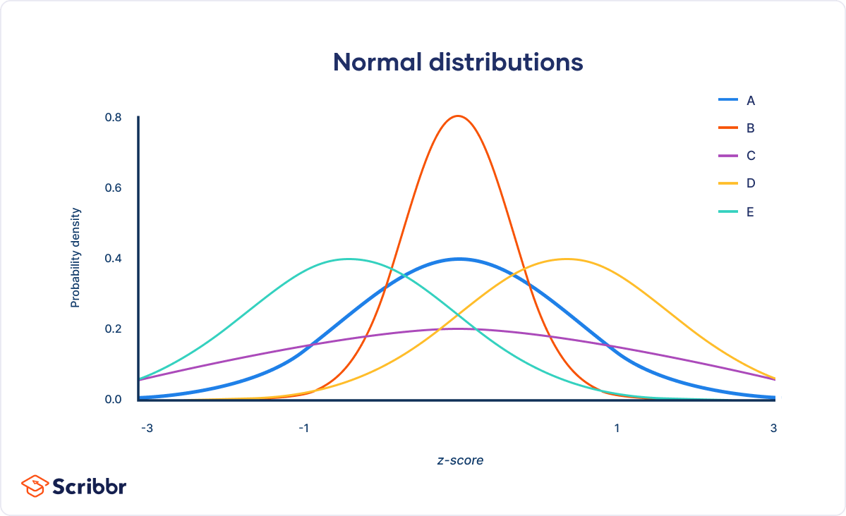
| Curve | Position or shape (relative to standard normal distribution) |
|-------|--------------------------------------------------------------|
| A (M = 0, SD = 1) | Standard normal distribution |
| B (M = 0, SD = 0.5) | Squeezed, because SD < 1 |
| C (M = 0, SD = 2) | Stretched, because SD > 1 |
| D (M = 1, SD = 1) | Shifted right, because M > 0 |
| E (M = –1, SD = 1) | Shifted left, because M < 0 |
 [☞(For image Reference, click here)](https://www.scribbr.com/statistics/standard-normal-distribution/)
## Standardizing a normal distribution
- When you standardize a normal distribution, the mean becomes 0 and the standard deviation becomes 1. This allows you to easily calculate the probability of certain values occurring in your distribution, or to compare data sets with different means and standard deviations.
- While data points are referred to as x in a normal distribution, they are called z or z scores in the z distribution. A z score is a standard score that tells you how many standard deviations away from the mean an individual value (x) lies:
- A positive z score means that your x value is greater than the mean.
- A negative z score means that your x value is less than the mean.
- A z score of zero means that your x value is equal to the mean.
[☞(For image Reference, click here)](https://www.scribbr.com/statistics/standard-normal-distribution/)
## Standardizing a normal distribution
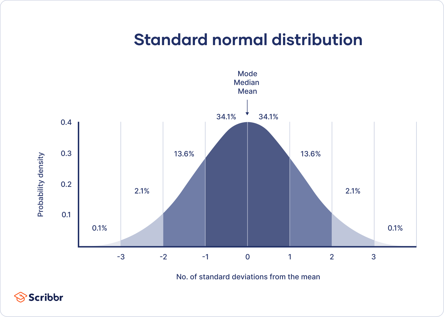
- When you standardize a normal distribution, the mean becomes 0 and the standard deviation becomes 1. This allows you to easily calculate the probability of certain values occurring in your distribution, or to compare data sets with different means and standard deviations.
- While data points are referred to as x in a normal distribution, they are called z or z scores in the z distribution. A z score is a standard score that tells you how many standard deviations away from the mean an individual value (x) lies:
- A positive z score means that your x value is greater than the mean.
- A negative z score means that your x value is less than the mean.
- A z score of zero means that your x value is equal to the mean.
 [☞(For image Reference, click here)](https://www.scribbr.com/statistics/normal-distribution/)
- **Formula:**
$z=\frac{x-\mu}{\sigma}$
where
- $x$ = individual value
- $\mu$ = mean
- $\sigma$ = standard deviation
[☞(For image Reference, click here)](https://www.scribbr.com/statistics/normal-distribution/)
- **Formula:**
$z=\frac{x-\mu}{\sigma}$
where
- $x$ = individual value
- $\mu$ = mean
- $\sigma$ = standard deviation